RALSA with R Markdown

Nowadays there is myriad of technologies for writing reproducible documents directly into R falling under the umbrella of R Markdown – plain R Markdown documents, more sophisticated R Bookdown documents and the newest framework of Quarto that uses not just R, but also other languages. In fact, documents with statistical computations in R can also be produced in plain LaTeX or via some R packages like tinytex. Whichever approach is used, the general idea is the same – write text, insert code chunks that compute on the data, present the results in tables and graphs, and add interpretations in text. This short guide presents a simple example on how to use R Markdown document to produce a PDF report containing graphs and tables and accompanying text. The approaches using LaTeX, R Bookdown and Quarto follow the same logic, although the actual implementation may slightly differ.

Since version 1.1.5 all analysis functions in RALSA can store outputs in object in the R environment rather than exporting them as MS Excel files (the default option). This is controlled by the save.output argument that needs to be set to FALSE.

To begin, we need to create a new R Markdown document in RStudio. Open RStudio and select File > New File > R Markdown. In the pop-up window select Document and change the default output format to PDF. Leave the rest of the settings as they are and save the document as Report.Rmd in a desired location on the hard drive. The new file comes with an yaml header that makes the basic definition of the document and its type and structure. These can be customized and made match the desired content and appearance. The default content with the yaml header on the top is displayed below.

---
title: "Untitled"
output: html_document
date: "2024-10-17"
---

```{r setup, include=FALSE}
knitr::opts_chunk$set(echo = TRUE)
```

## R Markdown
This is an R Markdown document. Markdown is a simple formatting syntax for authoring HTML, PDF, and MS Word
documents. For more details on using R Markdown see <http://rmarkdown.rstudio.com>.

When you click the **Knit** button a document will be generated that includes both content as well as the
output of any embedded R code chunks within the document. You can embed an R code chunk like this:

```{r cars}
summary(cars)
```

## Including Plots

You can also embed plots, for example:

```{r pressure, echo=FALSE}
plot(pressure)
```

Note that the `echo = FALSE` parameter was added to the code chunk to prevent printing of the R
code that generated the plot.

The first part of the document is the yaml header that instructs R Markdown on what the document type is, how to structure it, what is the title, date, and so on. Note the code chunks that start with ```{r...} and end with ```. These instruct R Markdown to perform computations, modify the outputs, present tables and graphs, etc. That is, these take data, compute on it and store the results like objects for further use. The plain parts of the text are actual text that will be displayed in the final compiled document. All lines that start with hashtags (#) are headings which will be displayed in the compiled document. Please refer to the RStudio’s introductory guide to R Markdown. There are many other resources available on the Internet on any of the topics related to R Markdown.

The final document content for this demonstration is displayed below.

---
title: |
| \vspace{-1.5cm}**Sample report produced with RALSA, knitr and Rmarkdown**
subtitle: |
| Analyzing Large-Scale Assessment Data using R
| A short demo on how to use R Markdown
| The John Smith University
output: pdf_document
classoption: a4paper
header-includes:
\usepackage[justification=raggedright,labelfont=bf,singlelinecheck=false]{caption}
urlcolor: red
linkcolor: red
author: \vspace{-0.85cm} John Smith
date: | 
| \vspace{-0.85cm}`r format(Sys.time(), '%B %d, %Y')`
---

```{r include = FALSE}
library(RALSA)
library(knitr)
```

```{r setup, include = FALSE}
knitr::opts_chunk$set(echo = TRUE)
```

<!-- Merge the data used in the examples below. -->
```{r, echo = FALSE, message = FALSE, warning = FALSE}
lsa.merge.data(inp.folder = "C:/Data/", file.types = list(asg = NULL), ISO = c("dnk", "swe", "fin", "nor"), out.file = "C:/Merged/Knitr_Merged_Data.RData")
```
This report presents the results from Nordic countries participating in TIMSS 2019, grade 4. The report is just a demo on how to use the `R` package [`RALSA`](https://ralsa.ineri.org). Besides the capability of saving the outputs in MS Excel format, the package also can store all outputs (tabular and graphical) into a list in the `R` environment.

Please note that the graphs produced by [`RALSA`](https://ralsa.ineri.org) are not using the basic plotting capabilities `R` comes with. Instead, the package uses `ggplot2` which allows to store the graphs as objects and then render them wherever needed in the document, as demonstrated here.

This document does not pretend to be an exhaustive guide on how to use [`RALSA`](https://ralsa.ineri.org) with the `knitr` package or any other of the R utilities to produce reports and presentations. It can be, however, be of help for anyone who likes working with `Rmarkdown` documents instead of generic word processing software as MS Word or the like. The same approach can be used with other documenting systems in `R` like Quarto or R Notebooks.You can use this document as a template and adjust it to your needs. The only thing I would ask you in return is to help me make the [`RALSA`](https://ralsa.ineri.org) package more popular among researchers.

## Student mathematics achievement by gender

Previous cycles of TIMSS have found that in most countries the mathematics achievement differs by gender. This study also looked into the achievement differences by gender. Table \ref{tab:pandoc_table_01} shows the mathematics achievement by gender in TIMSS 2019 in Nordic countries. The table also shows the number of sampled cases and their population estimate.

<!-- Compute the statistics. -->
```{r, echo = FALSE, message = FALSE, warning=FALSE}
pcts.means <- lsa.pcts.means(data.file = "C:/Merged/Knitr_Merged_Data.RData", split.vars = "ITSEX", PV.root.avg = "ASMMAT", graphs = TRUE, perc.x.label = "Student gender", perc.y.label = "Percentage of students", mean.x.labels = list("Student gender"), mean.y.labels = list("Average mathematics achievement"), save.output = FALSE)
```

<!-- Adding a table with achievement by gender from the output. -->
```{r, echo = FALSE, message = FALSE, warning=FALSE}

pcts.means[["Estimates"]][ , c("Mean_ASMMAT_SVR", "Mean_ASMMAT_MVR", "Variance_ASMMAT", "Variance_ASMMAT_SE", "Variance_ASMMAT_SVR", "Variance_ASMMAT_MVR", "SD_ASMMAT", "SD_ASMMAT_SE", "SD_ASMMAT_SVR", "SD_ASMMAT_MVR", "Percent_Missing_ASMMAT") := NULL]

pcts.means[["Estimates"]][ , c( "Sum_TOTWGT_SE", "Percentages_ITSEX", "Percentages_ITSEX_SE", "Mean_ASMMAT", "Mean_ASMMAT_SE") := lapply(.SD, function(i) {
as.numeric(format(round(x = i, digits = 2), nsmall = 2))
}), .SDcols = c( "Sum_TOTWGT_SE", "Percentages_ITSEX", "Percentages_ITSEX_SE", "Mean_ASMMAT", "Mean_ASMMAT_SE")]

data.table::setnames(pcts.means[["Estimates"]], c("Countries", "Gender", "n", "N", "(SE)", "Percentages", "(SE)", "Achievement", "(SE)"))

kable(pcts.means[["Estimates"]], format = "pandoc", caption = "Average overall mathematics achievement by gender.\\label{tab:pandoc_table_01}")
```

As the table shows, in all countries boys outperform girls. On average, boys have five points higher achievement. The largest difference is in Sweden (seven score points) and the smallest is in Finland (less than three score points). In general, however, the differences in all countries are small. The standard errors have to be considered in order to test these differences for their statistical significance. This report uses confidence intervals (see below), although more precise methods are available.

The distribution of students' overall mathematics achievement by their gender in each country is displayed graphically in the figures below. The figures represent 95% confidence intervals by gender. As can be seen in the figures, in none of the countries the difference is statistically significant. Even in Sweden (see Figure \ref{tab:pandoc_figure_04}) where the difference is the largest, it is not statistically significant.

<!-- Add figures from the output. -->
```{r, echo = FALSE, fig.cap = "Overal mathematics achievement by gender (Denmark)."}
pcts.means[["Means graphs"]][["Denmark"]][["Mean_ASMMAT"]]
```

```{r, echo = FALSE, fig.cap = "Overal mathematics achievement by gender (Finland)."}
pcts.means[["Means graphs"]][["Finland"]][["Mean_ASMMAT"]]
```

```{r, echo = FALSE, fig.cap = "Overal mathematics achievement by gender (Norway)."}
pcts.means[["Means graphs"]][["Norway"]][["Mean_ASMMAT"]]
```

```{r, echo = FALSE, fig.cap = "Overal mathematics achievement by gender (Sweden).\\label{tab:pandoc_figure_04}"}
pcts.means[["Means graphs"]][["Sweden"]][["Mean_ASMMAT"]]
```

A few things to note:

The first code chunk loads the necessary packages.
The second code chunk sets the options for all code chunks, forcing them to omit the standard R console output, so it is not included in the document.
Whatever computations are done, they are saved temporarily in the R environment for this document and then used for producing formatted tables and figures.
The outputs from computations using RALSA functions are stored in objects. These objects are lists. Further code chunks by the end of the document use these objects to extract and display only the necessary parts for presenting the results.

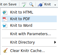
After the document is finalized, it needs to be compiled. Do so by clicking on the knitr icon in the top bar in RStudio. The document will compile and will be saved in the same folder where the R Markdown document was initially saved.

The compiled PDF file can be opened with any PDF viewer or editor.

RALSA – the R Analyzer for Large-Scale Assessments

This website provides resources on how to use the R Analyzer for Large-Scale Assessments (RALSA) to conduct analyses