
Table of contents
- Introduction
- The crosstabulation function and its arguments
- Computing crosstabulations using the command line
- Computing crosstabulations using the GUI
Introduction
The lsa.crosstabs function computes two-way tables between two categorical variables within groups of respondents defined by splitting variables. The splitting variables are optional. If no splitting variables are provided, the results will be computed on country level only. If splitting variables are provided, the data within each country will be split into groups by all splitting variables and the estimates will be computed by the categories of the last splitting variable. The estimates will be computed with the full weight and all of its replicates. At the end, their standard error computed using complex formulas which will depend on the study of interest. Whatever the estimate is, the standard error will be computed taking into account the complex sampling designs of the studies. Refer here for a short overview on the complex sampling designs of large-scale assessments and surveys. If interested in more in-depth details on the complex sampling and assessment designs of a particular study and how estimates and their standard errors are computed, refer to its technical documentation and user guide.
The function also computes the chi-square test of independence between row and column variables with the Rao-Scott design correction. When data from complex samples (as in large-scale assessments and surveys) are used, the traditional chi-square statistic is biased. The Rao-Scott adjustment provides unbiased estimates.
Like any other function in the RALSA package, the lsa.crosstabs function can recognize the study data and apply the correct estimation techniques given the study sampling and assessment design implementation without extra care.
The crosstabulations function and its arguments
The lsa.crosstabs function has the following arguments:
data.file– A file containinglsa.dataobject. Either this ordata.objectshall be specified, but not both. See details.data.object– The object in the memory containinglsa.data. Either this ordata.fileshall be specified, but not both. See details.split.vars– Categorical variable(s) to split the results by. If no split variables are provided, the results will be for the overall countries’ populations. If one or more variables are provided, the results will be split by all but the last variable and the percentages of respondents will be computed by the unique values of the last splitting variable.bckg.row.var– Name of the categorical background row variable. The results will be computed by all groups specified by the splitting variables. See details.bckg.col.var– Name of the categorical background column variable. The results will be computed by all groups specified by the splitting variables. See details.expected.cnts– Logical, shall the expected counts be computed as well? The default (TRUE) will compute the expected counts. IfFALSE, only the observed counts will be included in the output.row.pcts– Logical, shall row percentages be computed? The default (FALSE) will skip the computation of the row percentages.column.pcts– Logical, shall column percentages be computed? The default (FALSE) will skip the computation of the column percentages.total.pcts– Logical, shall percentages of total be computed? The default (FALSE) will skip the computation of the total percentages.weight.var– The name of the variable containing the weights. If no name of a weight variable is provided, the function will automatically select the default weight variable for the provided data, depending on the respondent type.include.missing– Logical, shall the missing values of the splitting variables be included as categories to split by and all statistics produced for them? The default (FALSE) takes all cases on the splitting variables without missing values before computing any statistics. See details.shortcut– Logical, shall the “shortcut” method for IEA TIMSS, TIMSS Advanced, TIMSS Numeracy, eTIMSS, PIRLS, ePIRLS, PIRLS Literacy and RLII be applied? The default (FALSE) applies the “full” design when computing the variance components and the standard errors of the estimates.graphs– Logical, shall graphs be produced? Default isFALSE.graph.row.label– String, custom label for the row variable in graphs. Ignored ifgraphs = FALSE.graph.col.label– String, custom label for the column variable in graphs. Ignored ifgraphs = FALSE.save.output– Logical, shall the output be saved in MS Excel file (default) or not (printed to the console or assigned to an object).output.file– Full path to the output file including the file name. If omitted, a file with a default file name “Analysis.xlsx” will be written to the working directory (getwd()).open.output– Logical, shall the output be open after it has been written? The default (TRUE) opens the output in the default spreadsheet program installed on the computer.
Notes:
- Either
data.fileordata.objectshall be provided as source of data. If both of them are provided, the function will stop with an error message. - The function computes two-way table by the categories of the splitting variables. The percentages of respondents in each group are computed within the groups specified by the last splitting variable. If no splitting variables are added, the results will be computed only by country.
- If
include.missing = FALSE(default), all cases with missing values on the splitting variables will be removed and only cases with valid values will be retained in the statistics. Note that the data from the studies can be exported in two different ways: (1) setting all user-defined missing values to NA; and (2) importing all user-defined missing values as valid ones and adding their codes in an additional attribute to each variable. If theinclude.missingis set toFALSE(default) and the data used is exported using option (2), the output will remove all values from the variable matching the values in itsmissingsattribute. Otherwise, it will include them as valid values and compute statistics for them. - The shortcut argument is valid only for TIMSS, TIMSS Advanced, TIMSS Numeracy, PIRLS, ePIRLS, PIRLS Literacy and RLII. Previously, in computing the standard errors, these studies were using 75 replicates because one of the schools in the 75 JK zones had its weights doubled and the other one has been taken out. Since TIMSS 2015 and PIRLS 2016 the studies use 150 replicates and in each JK zone once a school has its weights doubled and once taken out, i.e. the computations are done twice for each zone. For more details see the technical documentation and user guides for TIMSS 2015, and PIRLS 2016. If replication of the tables and figures is needed, the shortcut argument has to be changed to
TRUE. - If
graphs = TRUE, the function will produce graphs, heatmaps of counts per combination ofbckg.row.varandbckg.col.varcategory (population estimates) per group defined by thesplit.vars. All plots are produced per country. If nosplit.varsat the end there will be a heatmap for all countries together. If needed, custom horizontal and vertical axis labels can be defined using thegraph.row.labelandgraph.col.labelarguments. - TIMSS Longitudinal has two points of administration with the same sample of schools and, respectively, students. The teachers however, are not necessarily the same teachers in both administrations. When grade 4 teacher data is merged to student data, there are two sets of mathematics and science weights – one for the first year and one for the second year of administration. For grade 8, mathematics and science teachers have to be merged separately to student data, each having their own weights for the first and second year of administration. When analyses are performed, the first available weight is chosen as default. Student questionnaire items are available as two separate sets, one per year of administration. It is up to the analyst to choose the proper combination of items and weights for a particular analysis. For more details on the structure of the TIMSS Longitudinal database, see the TIMSS 2023 Longitudinal User Guide for the International Databse.
If save.output = FALSE, a list containing the estimates and analysis information. If graphs = TRUE, the plots will be added to the list of estimates. If save.output = TRUE (default), an MS Excel (.xlsx) file (which can be opened in any spreadsheet program), as specified with the full path in the output.file. If the argument is missing, an Excel file with the generic file name “Analysis.xlsx” will be saved in the working directory (getwd()).
The workbook contains four spreadsheets. The first one (“Estimates”) contains a table with the results by country and the final part of the table contains averaged results from all countries’ statistics. The following columns can be found in the table, depending on the specification of the analysis:
- <Country ID> – a column containing the names of the countries in the file for which statistics are computed. The exact column header will depend on the country identifier used in the particular study.
- <Split variable 1>, <Split variable 2>… – columns containing the categories by which the statistics were split by. The exact names will depend on the variables in
split.vars. - n_Cases – the number of cases in the sample used to compute the statistics for each split combination defined by the
split.vars, if any, and thebckg.row.var. - Sum_<Weight variable> – the estimated population number of elements per group after applying the weights. The actual name of the weight variable will depend on the weight variable used in the analysis.
- Sum_<Weight variable>_SE – the standard error of the the estimated population number of elements per group. The actual name of the weight variable will depend on the weight variable used in the analysis.
- Percentages_<Row variable> – the percentages of respondents (population estimates) per groups defined by the splitting variables in
split.vars, if any, and the row variable inbckg.row.var. The percentages will be for the combination of categories in the last splitting variable and the row variable which define the final groups. - Percentages_<Row variable>_SE – the standard errors of the percentages from above.
- Type – the type of computed values depending on the logical values passed to the
expected.cnts,row.pcts,column.pcts, andtotal.pctsarguments: “Observed count”, “Expected count”, “Row percent”, “Column percent”, and “Percent of total”. - <Column variable name Category 1>, <Column variable name Category 1>,… – the estimated values for all combinations between the row and column variables passed to
bckg.row.varandbckg.col.var. There will be one column for each category of the column variable. - <Column variable name Category 1, 2,… n>_SE – the standard errors of the estimated values from the above.
- Total – the grand totals for each of the estimated value types (“Observed count”, “Expected count”, “Row percent”, “Column percent”, and “Percent of total”) depending on the logical values (
TRUE,FALSE) passed to theexpected.cnts,row.pcts,column.pcts, andtotal.pctsarguments. - Total_SE – the standard errors of the estimated values from the above.
The second sheet contains some additional information related to the analysis per country in the following columns:
- <Country ID> – a column containing the names of the countries in the file for which statistics are computed. The exact column header will depend on the country identifier used in the particular study.
- <Split variable 1>, <Split variable 2>… – columns containing the categories by which the statistics were split by. The exact names will depend on the variables in
split.vars. - Statistics – contains the names of the different statistics types: chi-squares, degrees of freedom (sample and design), and p-values.
- Value – the estimated values for the statistics from above.
The third sheet contains some additional information related to the analysis per country in the following columns:
- DATA – used
data.fileordata.object. - STUDY – which study the data comes from.
- CYCLE – which cycle of the study the data comes from.
- WEIGHT – which weight variable was used.
- DESIGN – which resampling technique was used (JRR or BRR).
- SHORTCUT – logical, whether the shortcut method was used.
- NREPS – how many replication weights were used.
- ANALYSIS_DATE – on which date the analysis was performed.
- START_TIME – at what time the analysis started.
- END_TIME – at what time the analysis finished.
- DURATION – how long the analysis took in hours, minutes, seconds and milliseconds.
The fourth sheet contains the call to the function with values for all parameters as it was executed. This is useful if the analysis needs to be replicated later.
If graphs = TRUE there will be an additional “Graphs” sheet containing all plots.
If any warnings resulting from the computations are issued, these will be included in an additional “Warnings” sheet in the workbook as well.
Computing crosstabulations using the command line
In the examples that follow we will merge a new data file (see how to merge files here) with student and school principal data from PIRLS 2016 (Australia and Slovenia), taking all variables from both file types:
lsa.merge.data(inp.folder = "C:/temp",
               file.types = list(acg = NULL, asg = NULL),
               ISO = c("aus", "svn"),
               out.file = "C:/temp/merged/PIRLS_2016_ACG_ASG_merged.RData")
As a start, let’s compute a two-way table between two categorical variables – students’ sex (ASBG01) and how much students agree they like being at school (ASBG12A) in Australia and Slovenia. Variable ASBG01 has two valid categories: (1) “Girl”; and (2) “Boy”. Variable ASBG12A has four valid categories: (1) Agree a lot; (2) Agree a little; (3) Disagree a little; and (4) Disagree a lot. The student sex (ASBG01) will be the row variable and the agreement of students how much they like being at school (ASBG12A) will be the column variable in the table:
lsa.crosstabs(data.file = "C:/temp/PIRLS_2016_ACG_ASG_merged.RData",
              bckg.row.var = "ASBG01",
              bckg.col.var = "ASBG12A")
Few things to note:
- In international large-scale assessments all analyses must be done separately by country. There is no need, however, to add the country ID variable (IDCNTRY, or CNT in PISA) as a splitting variable. The function will identify it automatically and add it to the the vector of
split.vars. - There is no need to specify the weight variable explicitly. If no weight variable is specified explicitly, then the default weight (total student weight in this case) will be used for the data set depending on the merged respondents’ data, it is identified automatically. If you have a good reason to change the weight variable, you can do so by adding the
weight.var = "SENWGT", for example. - None of the additional arguments for computing the row percentages, column percentages and total percentages were specified. These can be computed as well, but the output becomes redundant and harder to read.
- Unless explicitly adding
save.output = FALSE, the output will be written to MS Excel on the disk. Otherwise, the output will be printed to the console. - If no output file is specified, then the output will be saved with “Analysis.xlsx” file name under the working directory (can be obtained with
getwd()). - Unless explicitly adding
open.output = FALSE, to the calling syntax, the output file will be opened after all computations are finished. This is useful when multiple calling syntaxes for different analyses are executed and no immediate inspection of the output is needed.
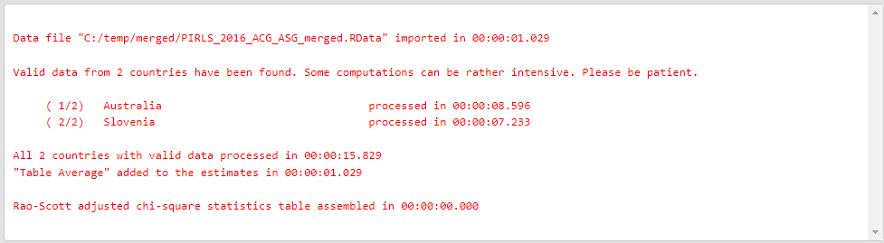
Executing the code from above will print the following output in the RStudio console:
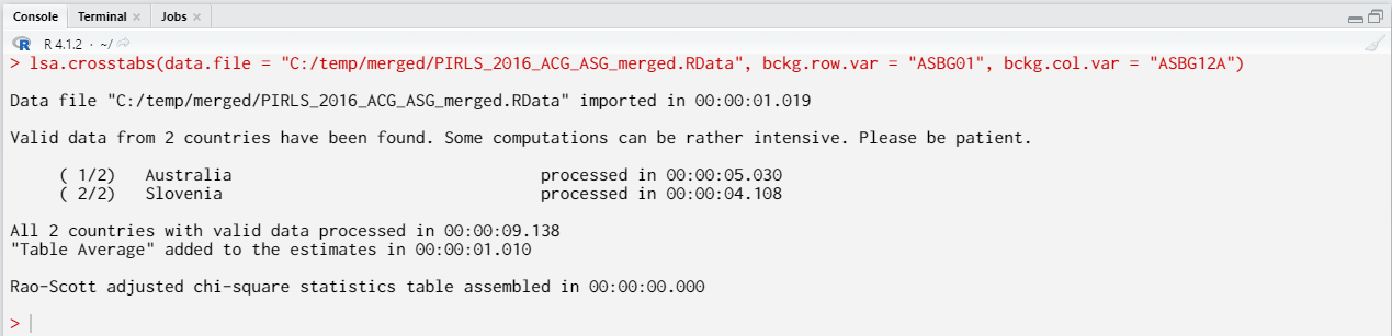
When all operations are finished the output will be written on the disk as MS Excel workbook. If open.output = TRUE (default), the file will be open in the default spreadsheet program (usually MS Excel). Refer to the explanations on the structure of the workbook, its sheets and the columns here.
Computing crosstabulations using the GUI
To start the RALSA user interface, execute the following command in RStudio:
ralsaGUI()
For the examples that follow, merge a new file with PIRLS 2016 data for Australia and Slovenia (Slovenia, not Slovakia) taking all student and school principal variables. See how to merge data files here. You can name the merged file PIRLS_2016_ACG_ASG_merged.RData.
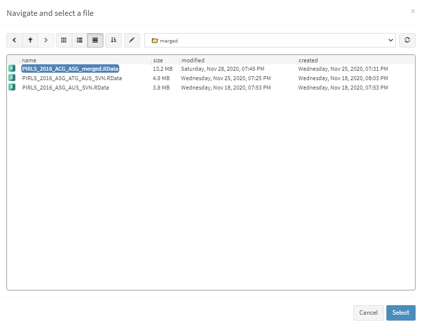
When done merging the data, select Analysis types > Crosstabulations from the menu on the left. When navigated to the Crosstabulations in the GUI, click on the Choose data file button. Navigate to the folder containing the merged PIRLS_2016_ACG_ASG_merged.RData file, select it and click the Select button.
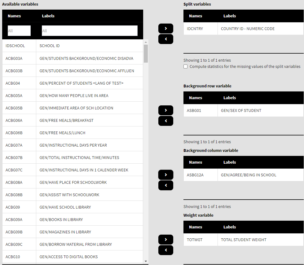
Once the file is loaded, you will see a panel on the left (available variables) and set of panels on the right where variables from the list of available ones can be added. We are going to compute a two-way table between two categorical variables – students’ sex (ASBG01) and how much students agree they like being at school (ASBG12A) in Australia and Slovenia. Variable ASBG01 has two valid categories: (1) “Girl”; and (2) “Boy”. Variable ASBG12A has four valid categories: (1) Agree a lot; (2) Agree a little; (3) Disagree a little; and (4) Disagree a lot. The student sex (ASBG01) will be the row variable and the agreement of students how much they like being at school (ASBG12A) will be the column variable in the table. Select variable ASBG01 from the list of Available variables and add them to the list of Background row variable using the right arrow button. Select variable ASBG12A from the list of Available variables and add them to the list of Background column variable using the right arrow button. This is all that needs to be done.
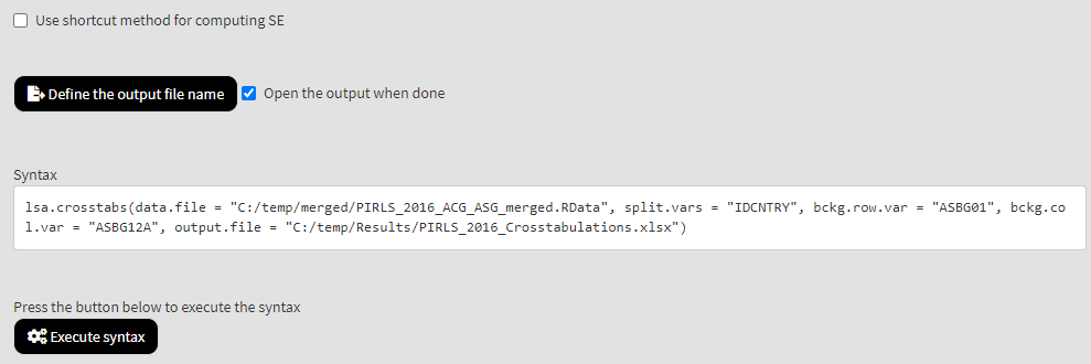
Scroll down and click on the Define output file name. Navigate to the folder C:/temp/Results (or to the folder where you want to save the output) and define the output file name. After you do so, a checkbox will appear next to the Define the output file name. If ticked, the output will open after all computations are finished. Underneath the calling syntax will be displayed. Under all of these the Execute syntax button will be displayed. The final settings in the lower part of the screen should look like this:
Click on the Execute syntax button. The GUI console will appear at the bottom and will log all completed operations:
Few things to note:
- In international large-scale assessments all analyses must be done separately by country. There is no need, however, to add the country ID variable (IDCNTRY, or CNT in PISA) as a splitting variable. The function will identify it automatically and add it to the the vector of
split.vars. - There is no need to specify the weight variable explicitly. If no weight variable is specified explicitly, then the default weight (total student weight in this case) will be used for the data set depending on the merged respondents’ data, it is identified automatically. If you have a good reason to change the weight variable, you can do so by adding the
weight.var = "SENWGT", for example. - None of the additional arguments for computing the row percentages, column percentages and total percentages were specified. These can be computed as well, but the output becomes redundant and harder to read.
- Unless explicitly unchecking the Open the output when done checkbox, the output file will be opened after all computations are finished.