Table of contents
- Introduction
- The continuous variables cutting function and its arguments
- Cutting continuous variables into discrete categorical using the command line
- Cutting continuous variables into discrete categorical using the GUI
Introduction
Often continuous variables need to be cut into categorical along the ranges of their values. For example, some continuous scales in large-scale assessments and surveys can be converted into two, three or more categories depending on the cut-points provided by the user. Examples of such cases are the complex background scales in TIMSS and PIRLS which are also provided as “index” variables with fixed categories in the form of “from-to”. This function cuts continuous variables into discrete ones using user-defined ranges. The resulting variables can be numeric or categorical (i.e. factors) depending on if value labels for the new values are provided.
The continuous variables cutting function and its arguments
The lsa.cut.vars function has the following arguments:
data.file– The file containinglsa.dataobject. Either this ordata.objectshall be specified, but not both. See details.data.object– The object in the memory containinglsa.dataobject. Either this ordata.fileshall be specified, but not both. See details.src.variables– Names of the variables to cut into categories. Accepts only continuous variables. No PV variables are accepted. See details.new.variables– The names of the new, cut variables to append to the dataset. See details.new.var.labels– Optional, vector of strings to add as variable labels for thenew.variables. See details.cut.points– Vector of numeric values to cut thesrc.variablesbetween. See details.value.labels– Optional, character vector of values to assign to the newly formed categorical discrete values in thenew.variables. See details.out.file– Full path to the.RDatafile to be written. If missing, the original object will be overwritten in the memory. See examples.
Notes:
- Either
data.fileordata.objectshall be provided as source of data. If both of them are provided, the function will stop with an error message. - The
src.variablesspecifies the variables that shall be cut. Only continuous variables are accepted. Multiplesrc.variablescan be passed. These will be split at the same cut points (see below). PVs are not accepted. - The
new.variablesargument is optional and specifies the names of the new discrete variables from thesrc.variables. The sequence of thenew.variablesnames is the same as thesrc.variables. If thenew.variablesargument is omitted, the function will create the names automatically, appendingCUTat the end of thesrc.variablesand store the discrete variable data under these names. If provided, the number ofnew.variablesmust be the same as the number ofsrc.variables. - The
new.var.labelsis optional. Regardless whethernew.variablesare provided, ifnew.var.labelsare provided, they will be assigned to thenew.variablesgenerated from the discretization. If neithernew.variablesnotnew.var.labelsare provided, the function will automatically generatenew.variables(see above) and copy the variable labels fromsrc.variablesto the newly generated variables, appendingCutat the beginning. The argument takes a vector with the same number of elements as the number of variable names insrc.variables. cut.pointsis a mandatory argument. It specifies the ranges (from-to) in the original variables to be cut into discrete categories. There can be multiplecut.points, the new values will be the ranges between them. For example, if the3.29309,7.97028,9.98618, and10.99411cut points are passed, there will be five categories in the resulting discrete variables, as follow:- From lowest up to
3.29309; - From above
3.29309up to7.97028; - From above
7.97028up to9.98618; - From above
9.98618up to10.99411; and - From above
10.99411to the highest value.
- From lowest up to
- The
cut.pointsmust be within the range of thesrc.variables. Otherwise the function will stop with an error. - The
value.labelsis optional. If omitted, the values in the new discrete variables will be numeric (integers). If the data was exported withmissing.to.NA = FALSE(i.e. user-defined missings are kept) the missing values will remain as they are. If thevalue.labelsare provided, the new values will be converted to factor levels. If the data was exported withmissing.to.NA = FALSEthe names of missing values will be assigned to factor levels too. Either way, the missing values will remain as missing values and handled properly by the analysis functions. Ifmissing.to.NA = TRUE(i.e. setting the user-defined missing values toNA), theNAvalues will remain asNAin the resulting discretenew.variables. - If full path to
.RDatafile is provided toout.file, the data.set will be written to that file. If no, the complemented data will remain in the memory. - A
lsa.dataobject in memory (ifout.fileis missing) or.RDatafile containinglsa.dataobject with the new discrete variables.
Cutting continuous variables into discrete categorical using the command line
In the examples that follow we will merge a new data file (see how to merge files here) with student data from PIRLS 2021 (Australia and Slovenia), taking all variables from both file types:
lsa.merge.data(inp.folder = "C:/temp",
               file.types = list(acg = NULL, asg = NULL),
               ISO = c("aus", "svn"),
               out.file = "C:/temp/merged/PIRLS_20221_ASG_merged.RData")
Note that the selected variables must be continuous, and not categorical. The variables also cannot be PVs. If any of these conditions is not met, the lsa.cut.vars will stop with error messages. So, let’s cut the Students Like Reading (ASBGSLR) and the Home Resources for Learning (ASBGHRL) continuous scales into discrete categorical variables. The cut points used for cutting the variable must be within the range of values of each source variables. To check the ranges (minimum and maximum values) of the source variables, use the lsa.data.diag function (you can see how to do this here).
As we now have the data from these two countries merged, we will cut the PIRLS 2021 Students Like Reading (ASBGSLR) and the Home Resources for Learning (ASBGHRL). The variables for these two scales in the database are continuous. Multiple variables can be cut into discrete ones at the same time, as in this example. In cutting them into discrete variables, we will assign labels for the discrete categories, as well as variable labels. Note that, as explained in the previous section, if we omit the new value labels, the resulting variables will contain numeric (integer) values. If these are provided, the variables will be set to categorical (factor) ones. If variable labels are provided, these will be assigned as descriptive labels for these variables. If omitted, the variable labels will be copied over from the source variables, adding “Cut” at the very front. The syntax below provides all these details. The source data file is overwritten with the data containing these two discretized variables.
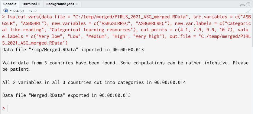
lsa.cut.vars(data.file = "C:/temp/merged/PIRLS_20221_ASG_merged.RData",
             src.variables = c("ASBGSLR", "ASBGHRL"),
             new.variables = c("ASBGSLRREC", "ASBGHRLREC"),
             new.var.labels = c("Categorical like reading", "Categorical learning resources"),
             cut.points = c(4.1, 7.9, 9.9, 10.7),
             value.labels = c("Very low", "Low", "Medium", "High", "Very high"),
             out.file = "C:/temp/merged/PIRLS_20221_ASG_merged.RData")
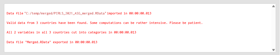
The call to this syntax will return the following output in the console:
If the data was exported with missing.to.NA = FALSE (i.e. user-defined missings are kept) the codes for the missing values will remain as they are and they will be marked as such, so that any other functions (data preparation or analysis) will treat them as missing values when using the data.
Cutting continuous variables into discrete categorical using the GUI
To start the RALSA user interface, execute the following command in RStudio:
ralsaGUI()
For the examples that follow, merge a new file with PIRLS 2021 data for Australia and Slovenia (Slovenia, not Slovakia) taking all student variables. See how to merge data files here. You can name the merged file PIRLS_2021_ASG_merged.RData.
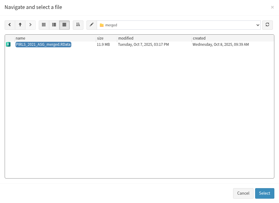
When done merging the data, select Data preparation > Cut variables from the menu on the left. When navigated to the Cut variables in the GUI, click on the Choose data file button. Navigate to the folder containing the merged PIRLS_2021_ASG_merged.RData file, select it and click the Select button.
Once the file is loaded, you will see the two panels with the available variables and selected variables (the latter is currently empty):
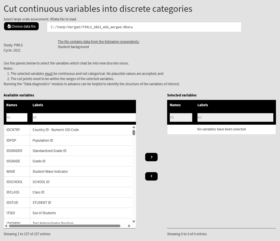
Use the mouse to select individual variables and the single arrow buttons to move them from the list of available variables to the list of selected variables and vice versa. You can use the filter boxes on the top of the panels to find the needed variables quickly. Note that the selected variables must be continuous, and not categorical. The variables also cannot be PVs. If any of these conditions is not met, the GUI will not let you continue any further and warnings will be displayed. So, let’s cut the Students Like Reading (ASBGSLR) and the Home Resources for Learning (ASBGHRL) continuous scales into discrete categorical variables. The cut points used for cutting the variable must be within the range of values of each source variables. To check the ranges (minimum and maximum values) of the source variables, use the Data diagnostics functionality of RALSA (you can see how to do this here). Find the variables for the two scales in the list of available variables on the left (you can use the filter at the top) and move it to the list of the selected variables. Once there are any variables in the Selected variables panel, the following will appear at the bottom of the screen:
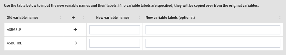
As the note on top states, each selected variable must have a new variable name for saving the data under it. The variable labels are short descriptions of the variable content. All or none shall be specified. If not specified, the variable labels will be copied over from the source variables, appending “Cut” at the beginning. After the information in the boxes above is completed, the following elements will appear at the bottom of the page:

In the text box, enter the cut points that will define the new categories. For this example, let’s enter 4.1, 7.9, 9.9, and 10.7. Enter them divided by spaces, no commas or other separators. Pressing the Reset button will clear all entered values. After entering the values, the following elements will appear:
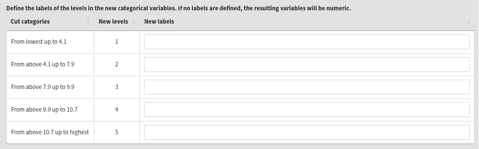
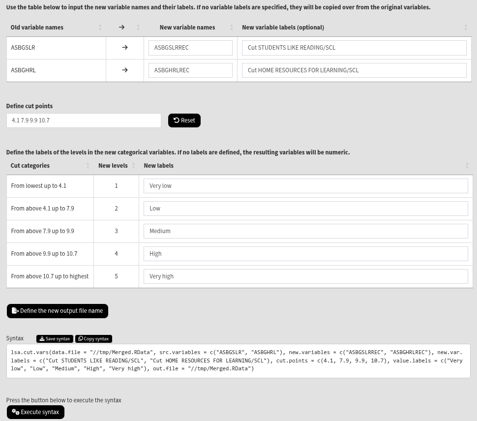
The table shows what will be the new categories will be. The new categories will be defined in ranges, according to the cut points, from below the lowest cut point to above the highest cut point. If no value labels are defined in the last column, the resulting new variables will be numeric (integers). If new value labels are defined, the resulting new variables will be categorical (factors). Enter the following labels from top to bottom: “Very low”, “Low”, “Medium”, “High”, and “Very high”. Press the Define the new output file name button, navigate to the folder where you want to save the new data file, define the file name and click on the Save button. In this case, we will define the same file name as the source file in the same location. This will overwrite the file, adding the new variables to it. The final screen should look like the image below:
Click on the Execute syntax button. The GUI console will appear at the bottom and will log all completed operations: