
Table of contents
Introduction
This section targets users who are not yet experienced with R and/or limited experience with large-scale assessment data. If you already have experience with these, feel free to skip it.
The workflow of RALSA goes as follow:
- Data preparation.
- Convert the SPSS (or TXT data in case of PISA cycles prior 2015). For every study cycle you need to do this just once. Then you can use the data for further data processing and/or analysis, not only in the current session, but also in other sessions.
- Merge data from different countries and respondents to analyze their data together.
- (Optional) Produce variable dictionaries. This is useful to see what are the properties of the variables in a converted and merged data set.
- (Optional) Recode variables. This can be useful to collapse/combine variables’ unique categories or to reverse the order of variables. It is particularly useful when performing binary logistic regression analysis because this type of analysis can use only a dichotomous variable as dependent.
- Perform analysis.
- Percentages and means; or
- Percentiles; or
- Benchmarks; or
- Correlations; or
- Linear regression; or
- Binary logistic regression.
We recommend using RStudio (a free and open-source IDE for R) because of its capabilities which ease the users.
RALSA can operate in two modes – through command line/script input and Graphical User Interface (GUI). Working with the command line where the user types statements by hand is the traditional way working with R and, at least for the experienced users, the most productive way in interacting with it.
R operates using packages. When you start R/RStudio, several packages are loaded by default. All other packages have to be loaded to use the functionality they add to R. Open RStudio and type the following in the console or the script editor:
install.packages("RALSA", dependencies = TRUE)
This will install the RALSA package from the CRAN repository or its mirrors. You need to do this just once. R packages receive updates frequently. To check for newer versions of the packages currently installed in R on your system, run the following command:
old.packages()
If you see that RALSA received an update, you can update it, along with all other liste packages, by running the following command:
update.packages(ask = FALSE)
This will update all packages on your system which received updates without asking for your permission for each one. Run the above commands regularly to keep your installed packages up to date.
Once you have installed RALSA, you can load the library using the following command:
library(RALSA)
This will attach the package to your path and will make all its functionality available to you, displaying some welcoming messages. You are ready to go, using all available functions.
Command line use
All functions in a package have an unique name. Start typing a command from the RALSA package, after adding few characters, RStudio will drop a menu where you will see a list of commands where you can choose the function you are interested in. Choose it with the mouse (or using the arrow keys on your keyboard and pres ↵). The command you started typing will be completed and opening and closing round brackets will be added at the end.
All (well, OK, almost all) functions in R have arguments. Arguments tell the function what you want it to do and/or how. Every argument is followed by an equal sign and value. Consider the following example. We will convert SPSS data into large-scale assessment native .RData files. This is the very first step which need to be done because studies do not provide their data sets in native R format, just in SPSS and SAS. After converting them, they can be used further to process the converted data (merge, recode, view variable dictionaries) and perform analysis. Find the code below, it converts PIRLS 2016 data from SPSS into native .RData sets:
lsa.convert.data(inp.folder = "E:/IDB/PIRLS_2016_IDB/Data/PIRLS",
                 ISO = c("aus", "svn"),
                 out.folder = "C:/temp")
The above code snippet calls the lsa.convert.data function. Three arguments are passed to it:
inp.folder– the input folder, tell the function where the SPSS files you want to convert are located. The function will use the SPSS files in this folder. Adapt this path to the folder where you have the source SPSS files stored.ISO– the Alpha-3 ISO 3166 country codes. You don’t need to know the background of the coding scheme of ISO 3166. These are unique three-letter codes which represent the abbreviated country names. These are the fourth, fifth and sixth characters in a data file name. In this example, “aus” represents Australia and “svn” represents Slovenia (note — Slovenia, not Slovakia!).out.folder– output folder, the folder where you would like to save the converted files. It is a good practice to be different than the input folder, otherwise the folder where the original SPSS files are located will become really messy. Adapt this path to the folder where you want the converted files to be stored.
Note how the file paths are passed to inp.folder and out.folder — R does not accept backward slashes (\) in file paths. These are reserved special characters. R uses the UNIX convention of forward slashes (/), so when you paste the path, just change all the backward slashes with forward ones. You need to do this only when you use MS Windows, Linux and MacOS are UNIX-like systems and use forward slashes in the file paths.
This function has other arguments as well (see the reference manual) which were not passed to this call. These arguments have default values and if you are feeling OK with these default values, you don’t need to pass them to the function call.
Select the lines of the syntax and press Ctrl+Enter from your keyboard. RStudio will execute the code and will convert the SPSS files from the source folder and will store the converted .RData files in the output folder. While executing, the function will print output in the RStudio console: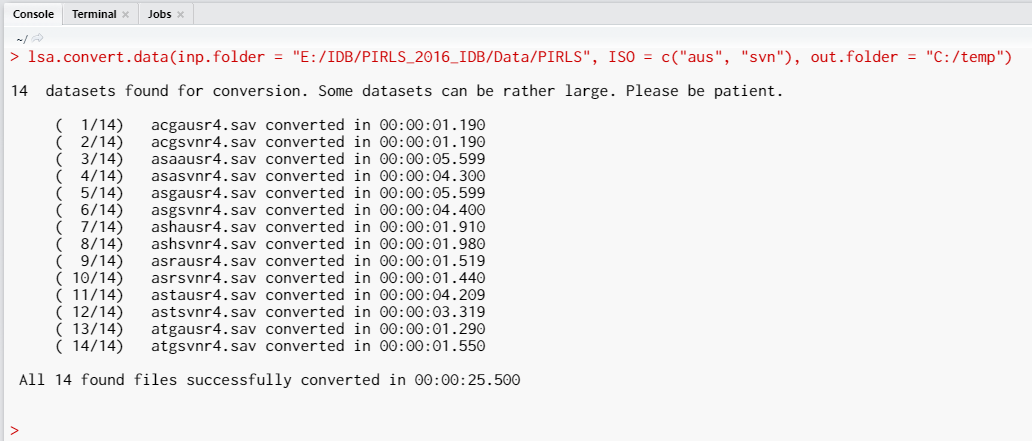
The output in the console reports the sequential number of files out of total number of files, the times needed to convert each file and the total time needed for all files you chose.
The above example shows the common working routine for all functions. Of course, the number and type of arguments for every function will be different, but this is the general workflow.
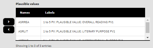
A special note has to be made on the use of “plausible values” (PVs). As shortly described here, the PVs are the achievement scores on the tested subject but, differently from the usual test scores, they represent more more than one score because of the test design. For example, for PIRLS 2016 the overall reading score will have five PVs: “ASRREA01”, “ASRREA02”, “ASRREA03”, “ASRREA04”, and “ASRREA05”. In PISA 2018 the overall mathematics will have thee following 10 PVs: “PV1MATH”, “PV2MATH”, “PV3MATH”, “PV4MATH”, “PV5MATH”, “PV6MATH”, “PV7MATH”, “PV8MATH”, “PV9MATH”, and “PV10MATH”. When computing any statistics involving achievement scores, all of the PVs for a certain score have to be used. PISA 2015 and later includes 10 PVs, all other studies include five. The statistics are computed with each PV and the final estimates and their standard errors are computed by aggregating all individual PV estimates using complex formulas. The interface will always show only the root of each set of PVs:
- For TIMSS (also preTIMSS and eTIMSS), PIRLS (also prePIRLS and ePIRLS), RLII, TIMSS Advanced and TiPi these will be shown as “ASRREA”, “ASRLIT”, “ASMMAT”, etc., i.e. stripping the numbers at the end of each PV in the set of PVs;
- For PISA, ICCS and ICILS these will be shown as “PV#MATH”, “PV#READ”, “PV#CIV”, etc., i.e. replacing the numbers within the root with “#”.
So, this is how these are going to look like in an analysis function (say lsa.pcts.means with PIRLS 2016 student and school principal data) for the first ones from above:
lsa.pcts.means(data.file = "C:/temp/PIRLS_2016_ACG_ASG_merged.RData",
               split.vars = "ITSEX", PV.root.avg = "ASRREA",
               output.file = "C:/temp/PIRLS_2016_Percentages_and_Means.xlsx")
And this is how they are going to look for the second (say lsa.pcts.means with PISA 2018 student data):
lsa.pcts.means(data.file = "C:/temp/cy07_msu_stu_qqq.RData",
               split.vars = "ST004D01T", PV.root.avg = "PV#MATH",
               output.file = "C:/temp/PISA_2018_Percentages_and_Means.xlsx")
Using the GUI
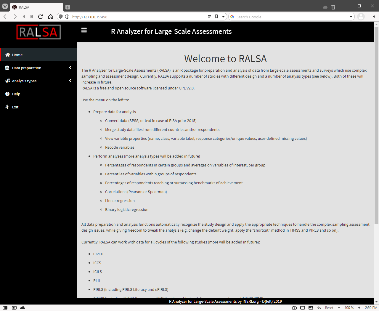
As stated earlier, traditionally R operates through command line. However, since a number of years R also provides the tools to construct graphical user interfaces. RALSA provides a user interface. For quick introduction on how to start and use the GUI watch the video below. The details are provided further.

The GUI can be started by executing the following command in the RStudio console:
ralsaGUI()
This will start the GUI in your default browser. The initial screen after the GUI is loaded will look like this:
Note: With future updates certain parts of the GUI may look different from the presentation here.
If you need to adjust the size of the GUI elements, hold the Ctrl key on the keyboard and scroll up and down with the mouse until you get the best view.
Use the menu on the left. When you click on Data preparation and Analysis types they will expand and offer you different options:
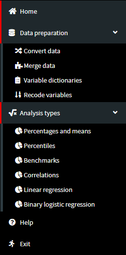
The sub-items are quite self-explanatory. The first item under Data preparation is Convert data, which we already exercised in the previous section when we converted SPSS data to native .RData sets. All data preparation and analysis types functionalities operate the same way — select a folder or load data file and follow the instructions on the screen. At every step the GUI will tell you what to do further. If a condition in a given step is not satisfied, the GUI will display a warning and won’t let you continue further.
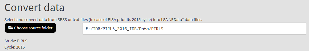
All of the different sections have common elements. The first common element you will see in most of the sub-menus under Data preparation is the Select source folder button. For example, when converting data, you need to select the directory which contains the SPSS (or TXT in case of PISA prior 2015 cycle) files you want to convert to native .RData files:
 Or, when selecting a file which you will use in computing certain type of statistics, you will need to choose a data file. This is an example for the Percentages and means analysis type where a data file needs to be loaded first, using the Choose data file button:
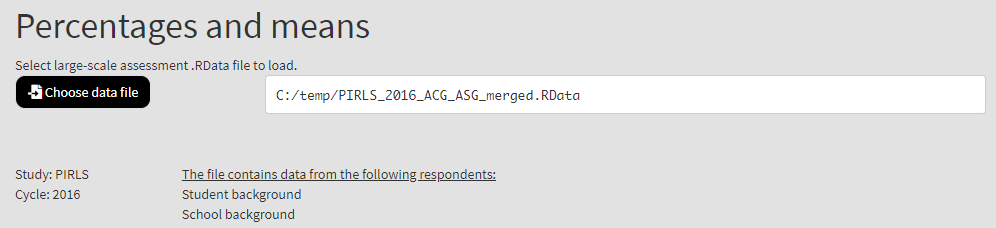
From the examples above notice that the study and cycle are recognized automatically. In the second example we also see data from which kinds of respondents are merged in the file.
A central common elements of the GUI are the ones enabling you to select items to include in the computations. For example, when converting data, after you pointed a directory containing SPSS files for a study, you will need to select countries whose data you would like to convert, as shown in the screenshot below:
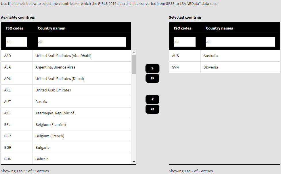
Use the right single arrow button to move individual countries you select from the list of available countries on the left to the list of selected countries on the right. Or conversely, if you have already have selected countries in the list of selected countries, use the left pointing arrow button to move them back to the list of available countries (i.e. deselect them). Use the left and right double arrow buttons to move all countries between the two lists.
A few more elements common to all sections in the GUI are displayed in the figure below.
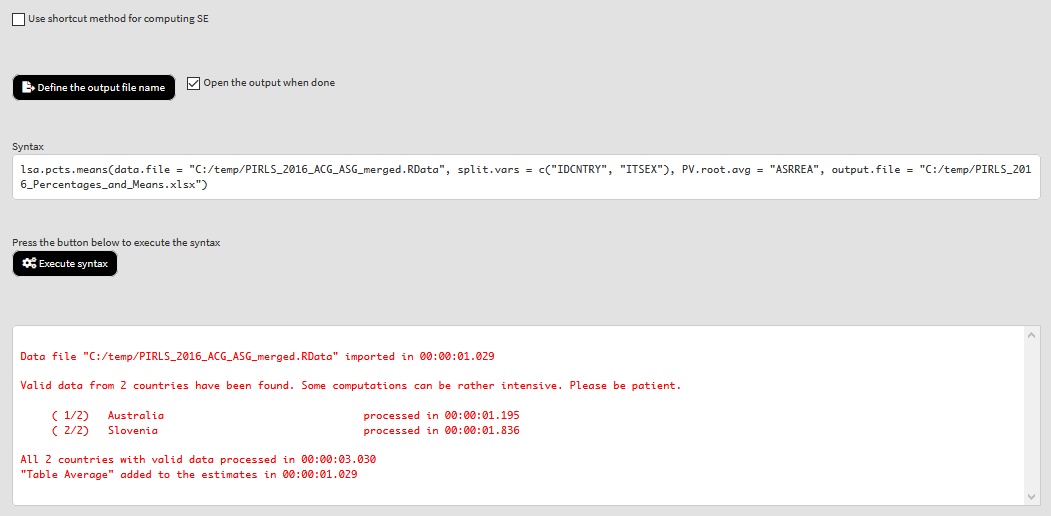
The first one is the Use shortcut method for computing SE checkbox. It will be shown only for the different analysis types, and only when TIMSS (also TIMSS Numeracy [a.k.a. preTIMSS] and eTIMSS), PIRLS (also PIRLS Literacy [a.k.a. prePIRLS] and ePIRLS) and the 2011 TIMSS and PIRLS joint study (a.k.a. TiPi) data is used in analysis. Prior TIMSS and PIRLS 2011 cycles the computation of the sampling error used 75 jackknife replication weights (i.e. one replicate weight for each jackknife replication zone). This is known as a “shortcut” method. Since their 2011 joint cycle TIMSS and PIRLS use 150 jackknife replicates (i.e. two replicate weights for each jackknife zone), known as the “full” method. The purpose of the implemented “shortcut” method in RALSA is to be able to replicate the estimates in the TIMSS and PIRLS international reports prior to 2011. We would recommend to always use the full method in the computations to obtain more precise estimates of the standard errors. For an overview of the sampling, measurement and the total errors of the estimates, see the studies’ technical documentation.
The second one is the Define the output file name button. Next to it is the Open the output when done. These two elements are common for all of the analysis types. The definition of the output file name is also available in the Merge data, Variable dictionaries, and Recode data in the Data preparation function section of RALSA while the Convert data will ask you to define output directory for the converted data. When you click on the button, you will be shown a file save dialog box. Navigate to the folder you would like to save the output file and define the file name for the output. The checkbox next to the button does what it says — the output MS Excel file will be opened when all computations are finalized.
Below the output file definition section you will see the calling syntax for the analysis (or data preparation). It is the same syntax that you would normally type by hand to prepare data or perform analysis. When you click on the Execute syntax button below it, the console displayed on the figure will show up and will show the progress of all operations.
Each sub-section in the Data preparation or Analysis types sections will have a number of other elements which are pertinent to them, but it will be too redundant to describe them here.
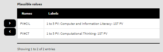
A special note has to be made on the use of “plausible values” (PVs). As shortly described here, the PVs are the achievement scores on the tested subject but, differently from the usual test scores, they represent more more than one score because of the test design. For example, for PIRLS 2016 the overall reading score will have five PVs: “ASRREA01”, “ASRREA02”, “ASRREA03”, “ASRREA04”, and “ASRREA05”. In PISA 2018 the overall mathematics will have thee following 10 PVs: “PV1MATH”, “PV2MATH”, “PV3MATH”, “PV4MATH”, “PV5MATH”, “PV6MATH”, “PV7MATH”, “PV8MATH”, “PV9MATH”, and “PV10MATH”. When computing any statistics involving achievement scores, all of the PVs for a certain score have to be used. PISA 2015 and later includes 10 PVs, all other studies include five. The statistics are computed with each PV and the final estimates and their standard errors are computed by aggregating all individual PV estimates using complex formulas. The interface will always show only the root of each set of PVs:
- For TIMSS (also preTIMSS and eTIMSS), PIRLS (also prePIRLS and ePIRLS), RLII, TIMSS Advanced and TiPi these will be shown as “ASRREA”, “ASRLIT”, “ASMMAT”, etc., i.e. stripping the numbers at the end of each PV in the set of PVs;
- For PISA, ICCS and ICILS these will be shown as “PV#MATH”, “PV#READ”, “PV#CIV”, etc., i.e. replacing the numbers within the root with “#”.
So, this is how these are going to look like in the interface for the first ones from above:
And this is how they are going to look for the second:
Give it a go and play around with it. Enjoy!