
Table of contents
- Introduction
- The data diagnostic tables function and its arguments
- Producing data diagnostic tables using the command line
- Producing data diagnostic tables using the GUI
| NOTE: This function is intended only as utility function for diagnostic purposes, to inspect the variables prior to performing an actual analysis. It is not intended for actual analysis of large-scale assessments' data. Reporting statistics from it can and will lead to biased and erroneous conclusions. |
Introduction
When performing an analysis, the properties of all included variables need to be known in advance. The lsa.vars.dict function (covered in the previous section) produces variable dictionaries which include information on the variable names, classes (numeric, factor, or character), labels, as well as their levels (i.e. response categories in case of factor variables) or unique values (in case of numeric or character variables), and their user-defined missing values (if any). However, it is always worth knowing the actual content of the data — what is the frequency of each value in a variable (in case of categorical variables) or what is the mean, variance, standard deviation, etc. (in case of continuous variables). The lsa.data.diag function produces frequency (in case of categorical variables) and descriptive (in case of continuous variables) tables which can be inspected and make decisions for the actual analysis or for recoding variables. The function computes all statistics per variable and puts the tables in a MS Excel workbook with one sheet per variable. It also adds an “Index” sheet to the workbook for easier navigation. All results are computed by country. Converted .RData large-scale assessments’ files or files where different countries and/or respondent types are merged can be used. The function is also generalized to non-large-scale assessments’ data and can be used with any data.frame or data.table.
The data diagnostic tables function and its arguments
The lsa.data.diag function has the following arguments:
data.file– The file containinglsa.dataobject. Either this ordata.objectshall be specified, but not both.data.object– The object in the memory containinglsa.dataobject. Either this ordata.fileshall be specified, but not both.split.vars– Variable(s) to split the results by. If no split variables are provided, the results will be computed on country level (if weights are used) or samples (if no weights are used).variables– Names of the variables to compute statistics for. If the variables are factors or character, frequencies will be computed, and if they are numeric, descriptives will be computed, unlesscont.freq = TRUE.weight.var– The name of the variable containing the weights, if weighted statistics are needed. If no name of a weight variable is provided, the function will automatically select the default weight variable for the providedlsa.data, depending on the respondent type."none"is for unweighted statistics.cont.freq– Shall the values of the numeric categories be treated as categorical to compute frequencies for?include.missing– Shall theNAand user-defined missing values (if available) be included as splitting categories for the variables insplit.vars? The default isFALSE.output.file– Full path to the output file including the file name. If omitted, a file with a default file name “Analysis.xlsx” will be written to the working directory (getwd()).open.output– Logical, shall the output be open after it has been written? The default (TRUE) opens the output in the default spreadsheet program installed on the computer....– Further arguments.
Note:
This function is intended only as utility function for diagnostic purposes, to inspect the variables prior to performing an actual analysis. It is not intended for actual analysis of large-scale assessments’ data. Reporting statistics from it can and will lead to biased and erroneous conclusions.
Producing data diagnostic tables using the command line
In this example we will use the data file merged in the last example using the command line for all variables in the file (if we omit the var.names argument, the function will produce diagnostic tables for all variables in the file). In RStudio execute the following syntax:
lsa.data.diag(data.file = "C:/temp/merged/PIRLS_2016_ASG_ATG_AUS_SVN.RData")
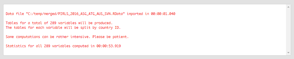
The call to the above syntax will return the following output in the console:
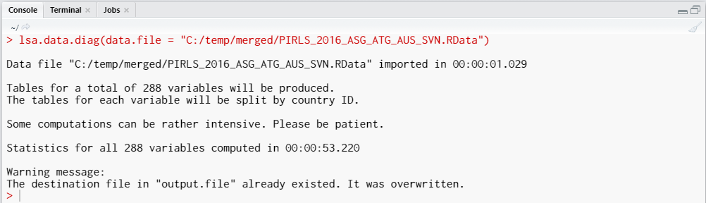
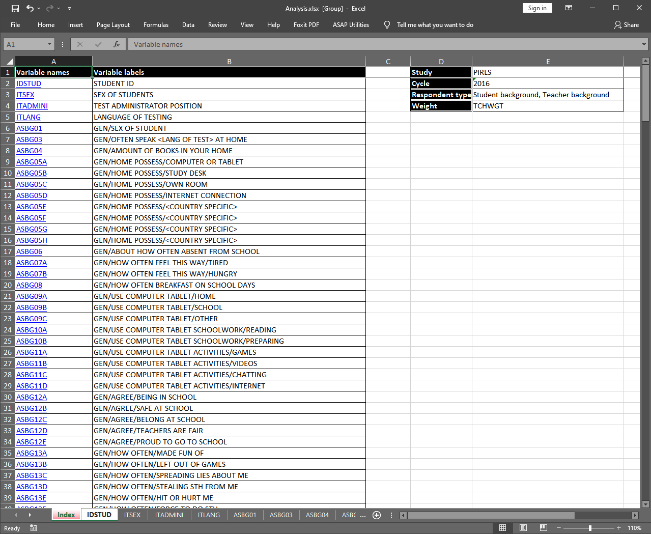
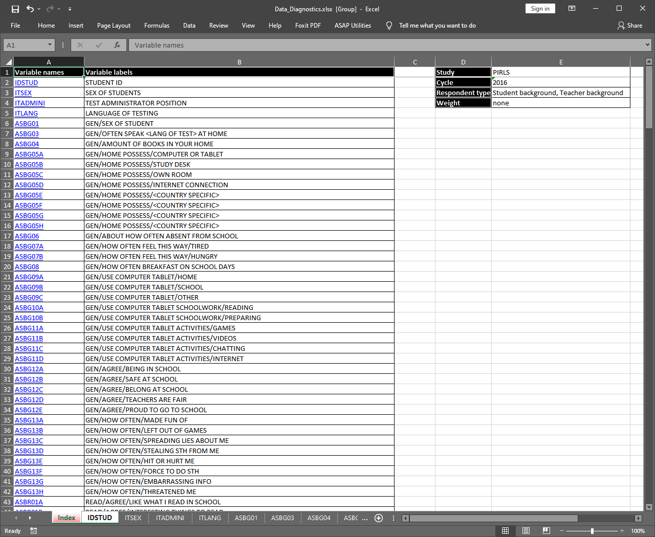
The exported MS Excel file with the “Index” sheet is shown on the figure below. The sheet contains information on the study, its cycle, the type(s) of respondent data (student and teacher in this case) and the used weight. In this case no weight was explicitly specified, so the function took the default one for this merged combination of respondents. We also did not specify a full path to the output file name, thus, a file named “Analysis.xlsx” is written to the working directory. The first two columns in the “Index” sheet contain the names and labels of the variables. Clicking on a variable name in the first column will switch to the sheet containing statistics for the corresponding variable.
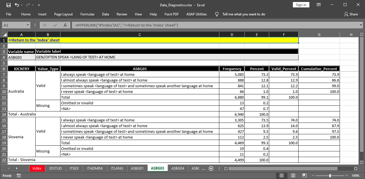
Let’s click on the link for variable ASBG03. The sheet for this variable is shown below.
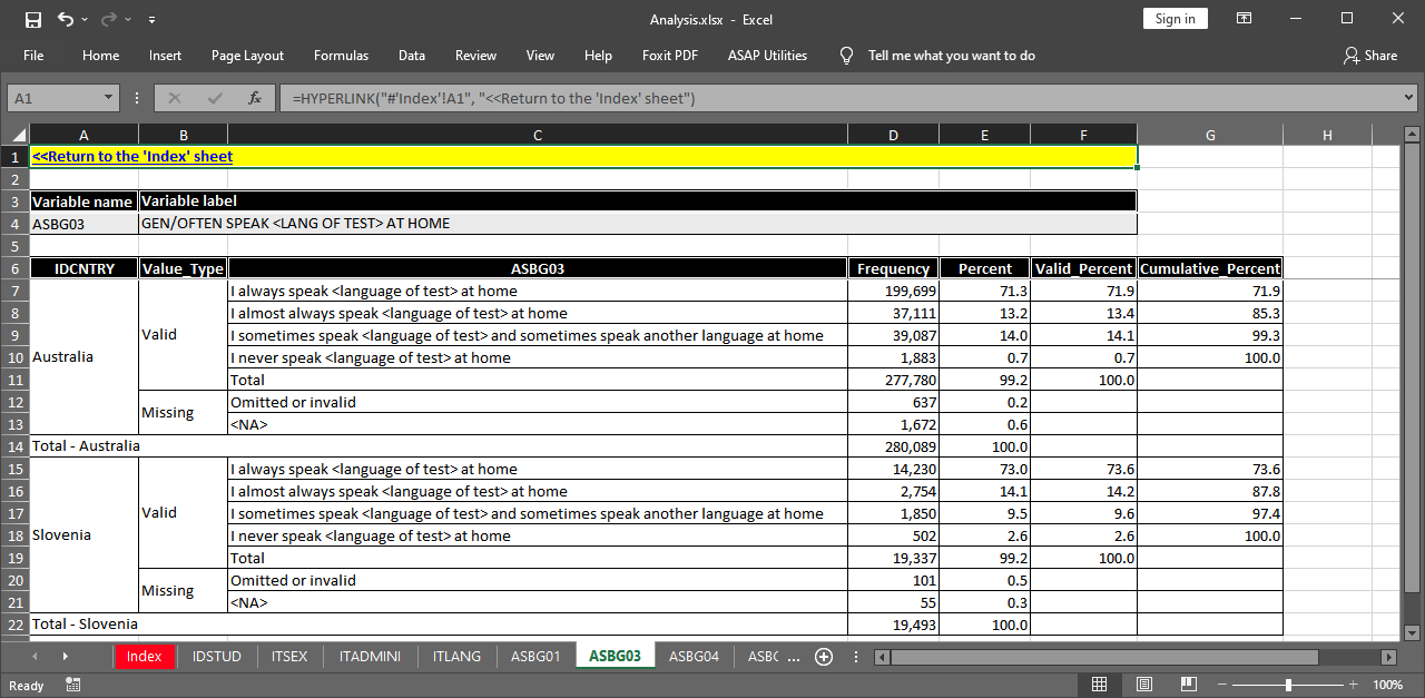
Note the yellow-shaded cell in the upper-left corner. It contains a link which allows to easily return to the “Index” sheet. The name and label for the variable are shown as well. The sheet shows the weighted frequencies, percentages, valid percentages and cumulative percentages. Note that we did not specify any splitting variables. The function automatically splits the results by country, even if the country ID variable is not specified as a splitting variable.
As a second example, let’s take just few variables – some categorical and some continuous. Let’s take student sex (ASBG01), student frequency of speaking the language of test at home (ASBG03), the teacher perception on safe and orderly school scale (ATBGSOS), and teachers’ job satisfaction scale (ATBGTJS). We will also split the results by teachers’ perceptions on parental involvement in school life (ATBG07F) in each country.
lsa.data.diag(data.file = "C:/temp/merged/PIRLS_2016_ASG_ATG_AUS_SVN.RData",
              split.vars = "ATBG07F",
              variables = c("ASBG01", "ASBG03", "ATBGSOS", "ATBGTJS"))
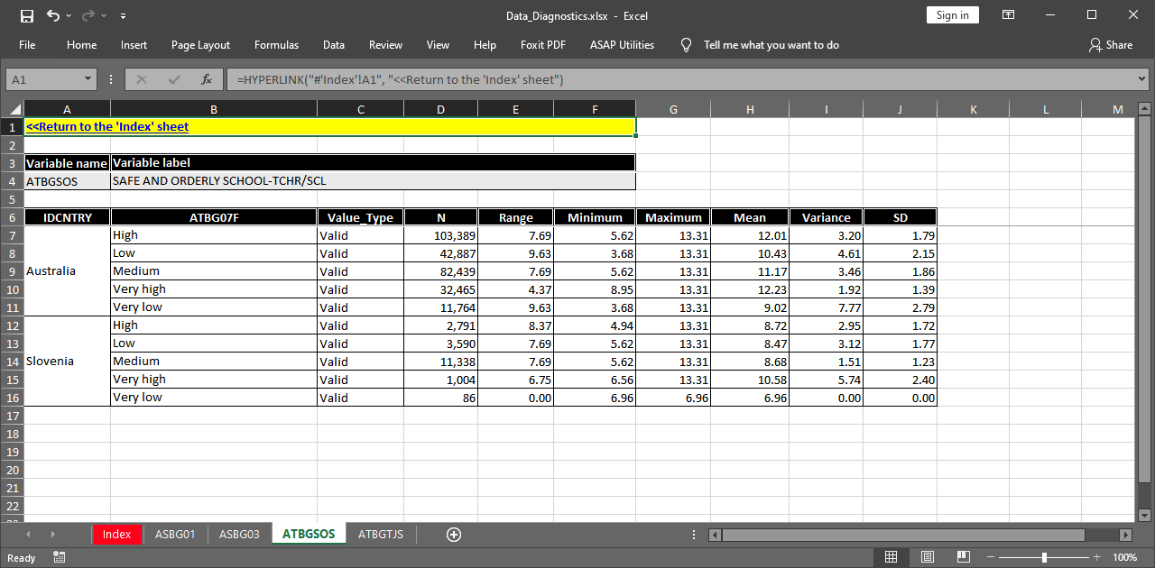
This time, the “Index” sheet contains rows for the variables we selected. Clicking on the cell with ATBGSOS link in the first column of the “Index” sheet takes us to the sheet containing the statistics for the “Safe and orderly school” teacher scale (continuous variable):
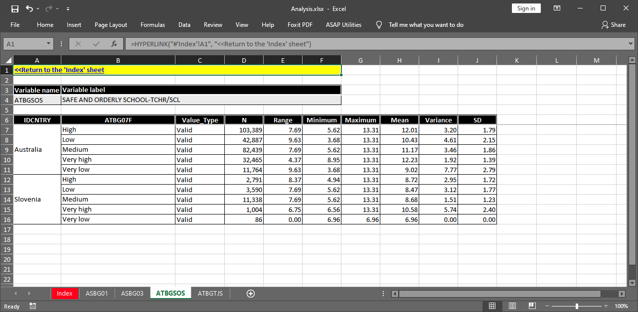
The variable is continuous, so instead of frequencies and percentages, the table shows the number of weighted cases, the range, minimum and maximum values, the mean, variance and standard deviation. This is the default behavior of the function. It can be overrode using the cont.freq argument. In this case the function will treat all continuous variables as categorical and will compute frequencies for each value.
Producing data diagnostic tables using the GUI
To start the RALSA user interface, execute the following command in RStudio:
ralsaGUI()
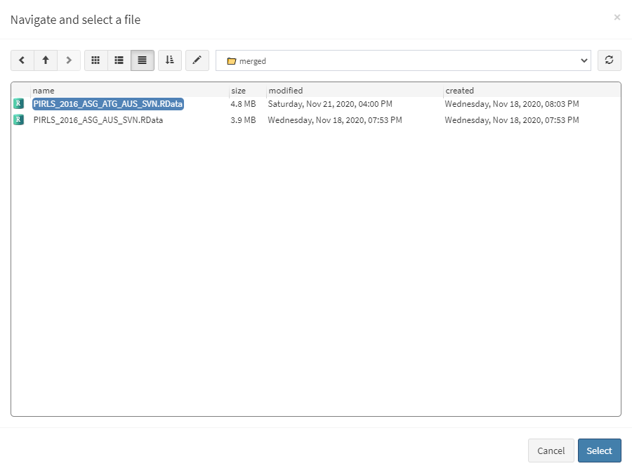
When the GUI opens in your browser, select Data preparation > Data diagnostics from the menu on the left. When navigated to the Data diagnostics in the GUI, click on the Choose data file button. Navigate to the folder containing the merged PIRLS_2016_ASG_ATG_AUS_SVN.RData file, select it and click the Select button.
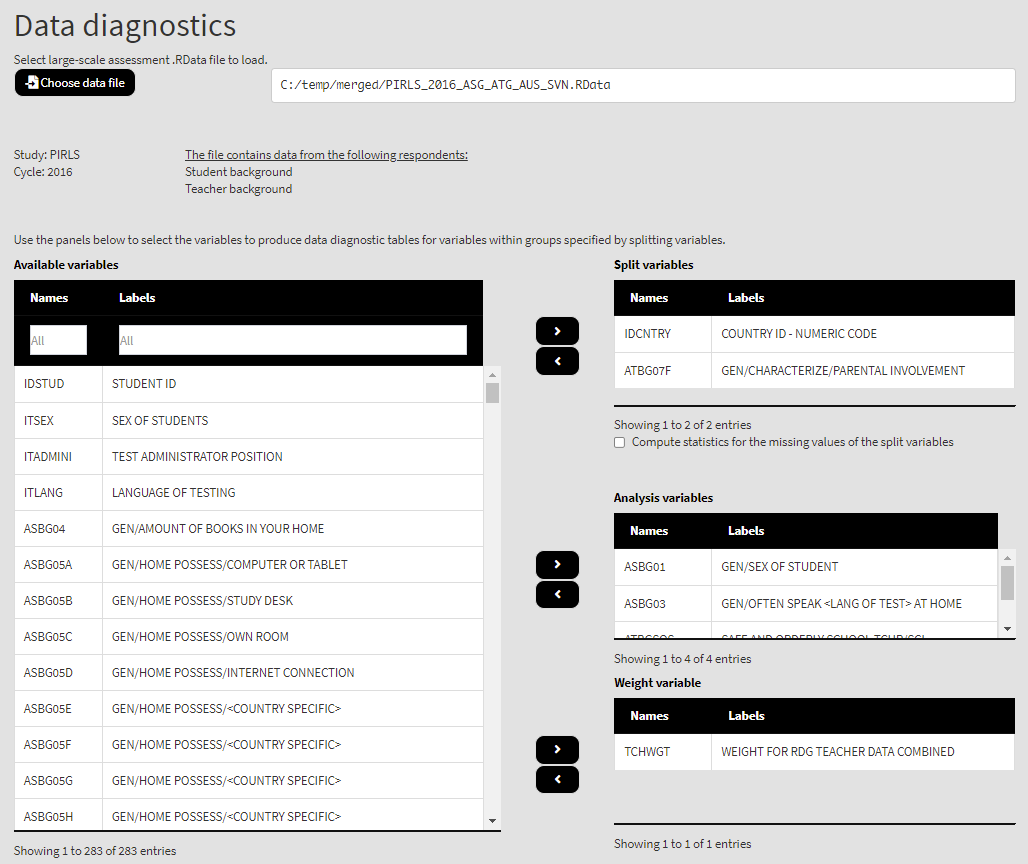
Once the file is loaded, you will see the two panels with the available variables and selected variables (the latter is currently empty):
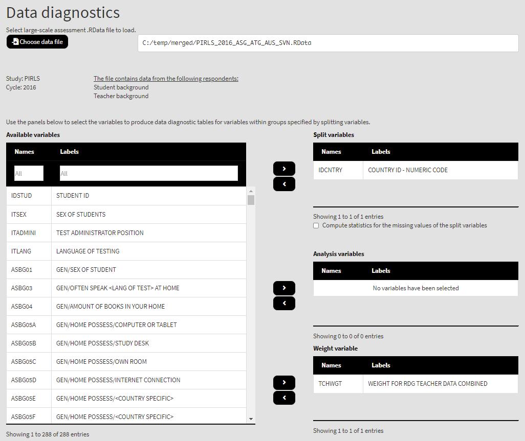
You can use the mouse to select individual variables and the single arrow buttons to move them from the list of available variables to the list of analysis and splitting variables and vice versa. The default weight is selected automatically, but it can be changed with another weight variable or no weight (the statistics will be unweighted). Use the single arrow buttons to select all or no variables. You can use the filter boxes on the top of the panels to find the needed variables quickly. Let’s select all available variables in the data file and move them to the list of Analysis variables. We will leave IDCNTRY (country ID variable) as the only splitting variable (default), so all results will be presented by country. The country ID cannot be removed from the list of Split variables. Once there are any variables in the Selected variables panel, the following elements will appear:
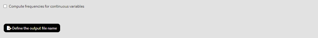
The if checkbox is ticked, it will tell RALSA that we want to treat the continuous variables as categorical and the frequencies, percentages, valid percentages and cumulative percentages for each value in the continuous variables instead of their total number of cases, ranges, minimum and maximum values, means, variances and standard deviations. We will leave the box unchecked. Press the Define the output file name button. Navigate to the folder C:/temp/Results (or to the folder where you want to save the output) and define the output file name. After you do so, a checkbox will appear next to the Define the output file name. If ticked, the output will open after all computations are finished. Underneath the calling syntax will be displayed. Under all of these the Execute syntax button will be displayed. The final settings in the lower part of the screen should look like this:
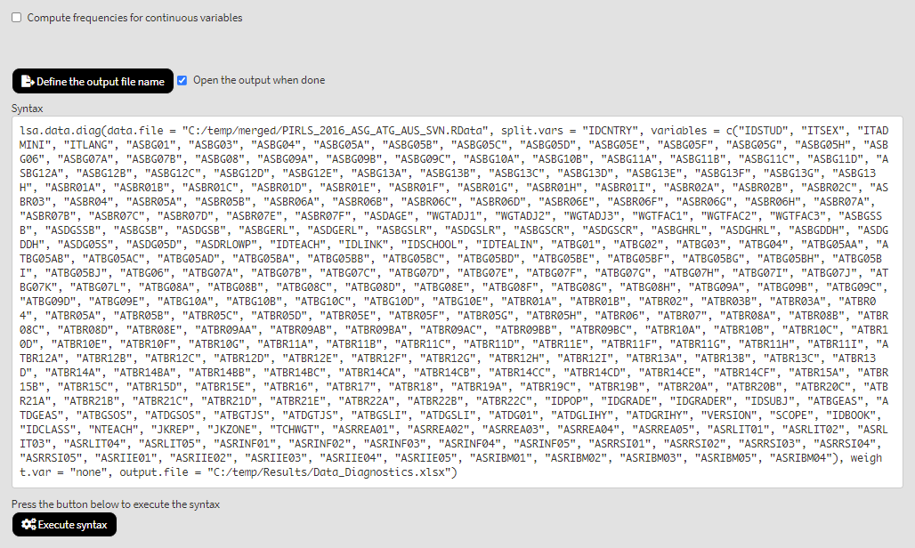
Click on the Execute syntax button. The GUI console will appear at the bottom and will log all completed operations:
If the Open the output when done checkbox is ticked, the output will open automatically in the default spreadsheet program (usually MS Excel) when all computations are completed. The exported MS Excel file with the “Index” sheet is shown on the figure below. The sheet contains information on the study, its cycle, the type(s) of respondent data (student and teacher in this case) and the used weight. In this case no weight was explicitly specified, so the function took the default one for this merged combination of respondents. The first two columns in the “Index” sheet contain the names and labels of the variables. Clicking on a variable name in the first column will switch to the sheet containing statistics for the corresponding variable.
Let’s click on the link for variable ASBG03. The sheet for this variable is shown below.
Note the yellow-shaded cell in the upper-left corner. It contains a link which allows to easily return to the “Index” sheet. The name and label for the variable are shown as well. The sheet shows the weighted frequencies, percentages, valid percentages and cumulative percentages. Note that we did not specify any splitting variables. All results are presented by country.
As a second example, let’s take just few variables – some categorical and some continuous. Let’s take student sex (ASBG01), student frequency of speaking the language of test at home (ASBG03), the teacher perception on safe and orderly school scale (ATBGSOS), and teachers’ job satisfaction scale (ATBGTJS). We will also split the results by teachers’ perceptions on parental involvement in school life (ATBG07F) in each country (you can move the selected variables from the Analysis variables panel one by one or refresh the browser which will reset the entire GUI and then load the data file again). Select the ATBG07F variable from the list of Available variables and add it to the list of Split variables. Select the ASBG01, ASBG03, ATBGSOS and ATBGTJS variables from the list of Available variables (you can use the filter boxes on the top) and add them to the Analysis variables. The final settings should look like this:
Define the output file name and execute the syntax. After all computations are finalized, the MS Excel workbook with the results will open automatically. This time, the “Index” sheet contains rows for the variables we selected. Clicking on the cell with ATBGSOS link in the first column of the “Index” sheet takes us to the sheet containing the statistics for the “Safe and orderly school” teacher scale (continuous variable):
The variable is continuous, so instead of frequencies and percentages, the table shows the number of weighted cases, the range, minimum and maximum values, the mean, variance and standard deviation. This is the default behavior of the function. It can be overrode by checking the Compute frequencies for continuous variables box. In this case the function will treat all continuous variables as categorical and will compute frequencies for each value.