
Table of contents
- Introduction
- The binary logistic regression function and its arguments
- Computing binary logistic regression coefficients using the command line
- Computing binary logistic regression coefficients using the GUI
Introduction
The lsa.bin.log.reg function computes logistic regression coefficients within groups of respondents defined by splitting variables where the dependent variable is binary (i.e. dichotomous, having just two distinct values). The splitting variables are optional. If no splitting variables are provided, the results will be computed on country level only. If splitting variables are provided, the data within each country will be split into groups by all splitting variables and the logistic regression coefficients will be computed for the last splitting variable. Independent variables can be both background/contextual variables and sets of PVs. All analyses will take into account the complex sampling and assessment design of the study of interest. When sets of PVs are used as independent variables, the logistic regression coefficients will be computed between the dependent variable and each PV in a set, and then the estimates for all PVs in the set will be averaged and their standard error computed using complex formulas which will depend on the study of interest. Refer here for a short overview on the complex sampling and assessment designs of large-scale assessments and surveys. If interested in more in-depth details on the complex sampling and assessment designs of a particular study and how estimates and their standard errors are computed, refer to its technical documentation and user guide.
Like any other function in the RALSA package, the lsa.bin.log.reg function can recognize the study data and apply the correct estimation techniques given the study sampling and assessment design implementation without extra care.
The binary logistic regression function and its arguments
The lsa.bin.log.reg function has the following arguments:
data.file– The file containinglsa.dataobject. Either this ordata.objectshall be specified, but not both.data.object– The object in the memory containinglsa.dataobject. Either this ordata.fileshall be specified, but not both.split.vars– Categorical variable(s) to split the results by. If no split variables are provided, the results will be for the overall countries’ populations. If one or more variables are provided, the results will be split by all but the last variable and the percentages of respondents will be computed by the unique values of the last splitting variable.bin.dep.var– Name of a binary (i.e. just two distinct values) background or contextual variable used as a dependent variable in the model.bckg.indep.cont.vars– Names of continuous independent background or contextual variables used as predictors in the model.bckg.indep.cat.vars– Names of categorical independent background or contextual variables used as predictors in the model to compute contrasts for (seebckg.cat.contrastsandbckg.ref.cats).bckg.cat.contrasts– Vector of integers with the same length as the length ofbckg.indep.cat.varsspecifying the type of contrasts to compute in casebckg.indep.cat.varsare provided.bckg.ref.cats– String vector with the same length as the length ofbckg.indep.cat.varsandbckg.cat.contrastsspecifying the reference categories for the contrasts to compute in casebckg.indep.cat.varsare provided.PV.root.indep– The root names for a set of plausible values used as a independent variables in the model.interactions– Interaction terms – a list containing vectors of length of two.standardize– Shall the dependent and independent variables be standardized to produce beta coefficients? The default isFALSE.weight.var– The name of the variable containing the weights. If no name of a weight variable is provide, the function will automatically select the default weight variable for the provided data, depending on the respondent type.norm.weight– Shall the weights be normalized before applying them, default isFALSE.include.missing– Logical, shall the missing values of the splitting variables be included as categories to split by and all statistics produced for them? The default (FALSE) takes all cases on the splitting variables without missing values before computing any statistics.shortcut– Logical, shall the “shortcut” method for IEA TIMSS, TIMSS Advanced, TIMSS Numeracy, eTIMSS, PIRLS, ePIRLS, PIRLS Literacy and RLII be applied? The default (FALSE) applies the “full” design when computing the variance components and the standard errors of the estimates.save.output– Logical, shall the output be saved in MS Excel file (default) or not
#’ (printed to the console or assigned to an object).output.file– Full path to the output file including the file name. If omitted, a file with a default file name “Analysis.xlsx” will be written to the working directory (getwd()).open.output– Logical, shall the output be open after it has been written? The default (TRUE) opens the output in the default spreadsheet program installed on the computer.
Notes:
- Either
data.fileordata.objectshall be provided as source of data. If both of them are provided, the function will stop with an error message. The function computes binary logistic regression coefficients by the categories of the splitting variables. The percentages of respondents in each group are computed within the groups specified by the last splitting variable. If no splitting variables are added, the results will be computed only by country. - If
standardize = TRUE, the variables will be standardized before computing any statistics to provide beta regression coefficients. - A binary (i.e. dichotomous) background/contextual variable must be provided to
bin.dep.var(numeric or factor). If more than two categories exist in the variable, the function will exit with an error. The function automatically recodes the two categories of thebin.dep.varto 0 and 1 if they are not as such (e.g. as 1 and 2 as in factors). If the variable of interest has more than two distinct values (can use thelsa.var.dictto see them), they can be collapsed using thelsa.recode.vars. - Background/contextual variables passed to
bckg.indep.cont.varswill be treated as numeric variables in the model. Variables with discrete number of categories (i.e. factors) passed tobckg.indep.cat.varswill be used to compute contrasts. In this case the type of contrast have to be passed tobckg.cat.contrastsand the number of the reference categories for each of thebckg.indep.cat.vars. The number of types of contrasts and the reference categories must be the same as the number ofbckg.indep.cat.vars. The currently supported contrast coding schemes are:dummy(also called “indicator” in logistic regression) – the odds ratios show what is the probability for a positive (i.e. 1) outcome in the binary dependent variable compared to the negative outcome (i.e. 0) per category of a variable in thebckg.indep.cat.catscompared to the reference category of that dummy coded variable. The intercept shows the log of the odds for the reference category when all other levels are 0.deviation(also called “effect” in logistic regression) – comparing the effect of each category (except for the reference) of the deviation coded variable to the overall effect (which is the intercept).simple– the same as for the dummy contrast coding, except for the intercept which in this case is the overall effect.
- Note that when using
standardize = TRUE, the contrast coding ofbckg.indep.cat.varsis not standardized. Thus, the regression coefficients may not be comparable to other software solutions for analyzing large-scale assessment data which rely on, for example, SPSS or SAS where the contrast coding of categorical variables (e.g. dummy coding) takes place by default. However, the model statistics will be identical. - Multiple continuous or categorical background variables and/or sets of plausible values can be provided to compute regression coefficients for. Please note that in this case the results will slightly differ compared to using each pair of the same background continuous variables or PVs in separate analysis. This is because the cases with the missing values are removed in advance and the more variables are provided, the more cases are likely to be removed. That is, the function support only listwisie deletion.
- Computation of regression coefficients involving plausible values requires providing a root of the plausible values names in
PV.root.depand/orPV.root.indep. All studies (except CivED, TEDS-M, SITES, TALIS and TALIS Starting Strong Survey) have a set of PVs per construct (e.g. in TIMSS five for overall mathematics, five for algebra, five for geometry, etc.). In some studies (say TIMSS and PIRLS) the names of the PVs in a set always start with character string and end with sequential number of the PV. For example, the names of the set of PVs for overall mathematics in TIMSS are BSMMAT01, BSMMAT02, BSMMAT03, BSMMAT04 and BSMMAT05. The root of the PVs for this set to be added toPV.root.deporPV.root.indepwill be “BSMMAT”. The function will automatically find all the variables in this set of PVs and include them in the analysis. In other studies like OECD PISA and IEA ICCS and ICILS the sequential number of each PV is included in the middle of the name. For example, in ICCS the names of the set of PVs are PV1CIV, PV2CIV, PV3CIV, PV4CIV and PV5CIV. The root PV name has to be specified inPV.root.deporPV.root.indepas “PV#CIV”. More than one set of PVs can be added inPV.root.indep. - The function can also compute two-way interaction effects between independent variables by passing a list to the
interactionsargument. The list must contain vectors of length two and all variables in these vectorsmust also be passed as independent variables. Note the following:- When an interaction is between two independent background continuous variables (i.e. both are passed to
bckg.indep.cont.vars), the interaction effect will be computed between them as they are. - When the interaction is between two categorical variables (i.e. both are passed to
bckg.indep.cat.vars), the interaction effect will be computed between each possible pair of categories of the two variables, except for the reference categories. - When the interaction is between one continuous (i.e. passed to
bckg.indep.cont.vars) and one categorical (i.e. passed tobckg.indep.cat.vars), the interaction effect will be computed between the continuous variable and each category of the categorical variable, except for the reference category. - When the interaction is between a continuous variable (i.e. passed to
bckg.indep.cont.vars) and a set of PVs (i.e. passed toPV.root.indep), the interaction effect is computed between the continuous variable and each PV in the set and the results are aggregated. - When the interaction is between a categorical variable (i.e. passed to
bckg.indep.cat.vars) and a set of PVs (i.e. passed toPV.root.indep), the interaction effect is computed between each category of the categorical variable (except the reference category) and each PV in the set. The results are aggregated for each of the categories of the categorical variables and the set of PVs. - When the interaction is between two sets of PVs (i.e. passed to
PV.root.indep), the interaction effect is computed between the first PV in the first set and the first PV in the second set, the second PV in the first set and the second PV in the second set, and so on. The results are then aggregated.
- When an interaction is between two independent background continuous variables (i.e. both are passed to
- If
norm.weight = TRUE, the weights will be normalized before used in the model. This may be necessary in some countries in some studies extreme weights for some of the cases may result in inflated estimates due to model perfect separation. The consequence of normalizing weights is that the number of elements in the population will sum to the number of cases in the sample. Use with caution. - If
include.missing = FALSE(default), all cases with missing values on the splitting variables will be removed and only cases with valid values will be retained in the statistics. Note that the data from the studies can be exported in two different ways: (1) setting all user-defined missing values to NA; and (2) importing all user-defined missing values as valid ones and adding their codes in an additional attribute to each variable. If theinclude.missingis set toFALSE(default) and the data used is exported using option (2), the output will remove all values from the variable matching the values in itsmissingsattribute. Otherwise, it will include them as valid values and compute statistics for them. - The shortcut argument is valid only for TIMSS, TIMSS Advanced, TIMSS Numeracy, PIRLS, ePIRLS, PIRLS Literacy and RLII. Previously, in computing the standard errors, these studies were using 75 replicates because one of the schools in the 75 JK zones had its weights doubled and the other one has been taken out. Since TIMSS 2015 and PIRLS 2016 the studies use 150 replicates and in each JK zone once a school has its weights doubled and once taken out, i.e. the computations are done twice for each zone. For more details see the technical documentation and user guides for TIMSS 2015, and PIRLS 2016. If replication of the tables and figures is needed, the shortcut argument has to be changed to
TRUE. The function provides two-tailed t-test and p-values for the regression coefficients. - Unless explicitly adding
save.output = FALSE, the output will be written to MS Excel on the disk. Otherwise, the output will be printed to the console. - If no output file is specified, then the output will be saved with “Analysis.xlsx” file name under the working directory (can be obtained with
getwd()).
The output produced by the function is stored in MS Excel workbook. The workbook has three sheets. The first one (“Estimates)” will have the following columns, depending on what kind of variables were included in the analysis:
- <Country ID> – a column containing the names of the countries in the file for which statistics are computed. The exact column header will depend on the country identifier used in the particular study.
- <Split variable 1>, <Split variable 2>… – columns containing the categories by which the statistics were split by. The exact names will depend on the variables in
split.vars. - n_Cases – the number of cases in the sample used to compute the statistics.
- Sum_<Weight variable> – the estimated population number of elements per group after applying the weights. The actual name of the weight variable will depend on the weight variable used in the analysis.
- Sum_<Weight variable>_SE – the standard error of the the estimated population number of elements per group. The actual name of the weight variable will depend on the weight variable used in the analysis.
- Percentages_<Last split variable> – the percentages of respondents (population estimates) per groups defined by the splitting variables in
split.vars. The percentages will be for the last splitting variable which defines the final groups. - Percentages_<Last split variable>_SE – the standard errors of the percentages from above.
- Variable – the variable names (background/contextual or PV root names, or contrast coded variable names). Note that when interaction terms are included, the cells with the interactions in the
Variablescolumn will contain the names of the two variables in each of the interaction terms, divided by colon, e.g.ASBGSSB:ASBGHRL. - Coefficients – the logistic regression coefficients (intercept and slopes).
- Coefficients_SE – the standard error of the logistic regression coefficients (intercepts and slopes) for each independent variable (background/contextual or PV root names, or contrast coded variable names) in the model.
- Coefficients_SVR – the sampling variance component for the logistic regression coefficients if root PVs are specified either as dependent or independent variables.
- Coefficients_<root PV>_MVR – the measurement variance component for the logistic regression coefficients if root PVs are specified either as dependent or independent variables.
- Wald_Statistic – Wald (z) statistic.
- p_value – the p-value for the regression coefficients.
- Odds_Ratio – the odds ratios of the logistic regression.
- Odds_Ratio_SE – the standard errors for the odds ratios of the logistic regression.
- Wald_L95CI – the lower 95% model-based confidence intervals for the logistic regression coefficients.
- Wald_U95CI – the upper 95% model-based confidence intervals for the logistic regression coefficients.
- Odds_L95CI – the lower 95% model-based confidence intervals for the odds ratios.
- Odds_U95CI – the upper 95% model-based confidence intervals for the odds ratios.
The second sheet (“Model statistics”) contains the statistics related to the binary logistic regression model itself in the following columns:
- <Country ID> – a column containing the names of the countries in the file for which statistics are computed. The exact column header will depend on the country identifier used in the particular study.
- <Split variable 1>, <Split variable 2>… – columns containing the categories by which the statistics were split by. The exact names will depend on the variables in
split.vars. - Statistic – a column containing the Null Deviance (-2LL, no predictors in the model, just constant, also called “baseline”), Deviance (-2LL, after adding predictors, residual deviance, also called “new”), DF Null (degrees of freedom for the null deviance), DF Residual (degrees of freedom for the residual deviance), Akaike Information Criteria (AIC), Bayesian information criterion (BIC), model Chi-Square, different R-Squared statistics (Hosmer & Lemeshow – HS, Cox & Snell – CS, and Nagelkerke – N).
- Estimate – the numerical estimates for each of the above.
- Estimate_SE – the standard errors of the estimates from above.
- Estimate_SVR – the sampling variance component if PVs were included in the model.
- Estimate_MVR – the measurement variance component if PVs were included in the model.
The third sheet (“Analysis information”) contains some additional information related to the analysis per country in the following columns:
- DATA – used
data.fileordata.object. - STUDY – which study the data comes from.
- CYCLE – which cycle of the study the data comes from.
- WEIGHT – which weight variable was used.
- DESIGN – which resampling technique was used (JRR or BRR).
- SHORTCUT – logical, whether the shortcut method was used.
- NREPS – how many replication weights were used.
- ANALYSIS_DATE – on which date the analysis was performed.
- START_TIME – at what time the analysis started.
- END_TIME – at what time the analysis finished.
- DURATION – how long the analysis took in hours, minutes, seconds and milliseconds.
The fourth sheet (“Calling syntax”) contains the call to the function with values for all parameters as it was executed. This is useful if the analysis needs to be replicated later.
Computing binary logistic regression coefficients using the command line
In the examples that follow we will merge a new data file (see how to merge files here) with student and school principal data from PIRLS 2016 (Australia and Slovenia), taking all variables from both file types:
lsa.merge.data(inp.folder = "C:/temp",
               file.types = list(acg = NULL, asg = NULL),
               ISO = c("aus", "svn"),
               out.file = "C:/temp/merged/PIRLS_2016_ACG_ASG_merged.RData")
As a start, let’s compute the binary logistic regression coefficients for a model to predict if students would agree or disagree that teachers treat them fair (variable ASBG12D) as a function of their own sense of school belonging (ASBGSSB, check the PIRLS 2016 technical documentation on how this scale is constructed and its properties) in Australia and Slovenia. The lsa.bin.log.reg function accepts only binary (i.e. dichotomous) variables as dependent, while the responses on the question of how much students agree or disagree that teachers treat them fair (ASBG12D) are organized into four distinct categories:
- Agree a lot
- Agree a little
- Disagree a little
- Disagree a lot
Thus, the first thing we need to do is to recode ASBG12D collapsing the categories into two where the “Disagree a lot” and “Disagree a little” are recoded as the first category, and “Agree a lot” and “Agree a little” as the second category:
lsa.recode.vars(data.file = "C:/temp/merged/PIRLS_2016_ACG_ASG_merged.RData",
                src.variables = "ASBG12D",
                old.new = "1=2;2=2;3=1;4=1;5=3",
                new.variables = "ASBG12Dr",
                new.labels = c("Disagree", "Agree", "Omitted or invalid"),
                missings.attr = "Omitted or invalid",
                variable.labels = "GEN/AGREE/TEACHERS ARE FAIR - RECODED",
                out.file = "C:/temp/merged/PIRLS_2016_ACG_ASG_merged.RData")
Note that we are recoding ASBG12D into a new variable (ASBG12Dr). This is recommended because we will keep the original variable ASBG12D as it is. We also assign a variable label to the newly created variable. Let’s compute the logistic regression coefficients using the new variable as dependent and ASBGSSB as independent:
lsa.bin.log.reg(data.file = "C:/temp/merged/PIRLS_2016_ACG_ASG_merged.RData",
                bin.dep.var = "ASBG12Dr",
                bckg.indep.cont.vars = "ASBGSSB")
Few things to note:
- The function can take one binary variable as dependent. The independent variables can be multiple background/contextual variables and/or sets of PVs. If PVs are included as independent variables, each set of PVs will be represented by their root name. For example, the five PVs for the overall reading achievement are ASRREA01, ASRREA02, ASRREA03, ASRREA04, and ASRREA05. In the
PV.root.corrargument we need to specify only the root of the PVs, “ASRREA”. The function will use this root/common name to select all five PVs and include them in the computations. For more details on the PV roots (also for the PV roots for studies other than TIMSS and PIRLS and their additions), the computational routines involving PVS, see here. - In international large-scale assessments all analyses must be done separately by country. There is no need, however, to add the country ID variable (IDCNTRY, or CNT in PISA) as a splitting variable. The function will identify it automatically and add it to the the vector of
split.vars. - There is no need to specify the weight variable explicitly. If no weight variable is specified explicitly, then the default weight (total student weight in this case) will be used for the data set depending on the merged respondents’ data, it is identified automatically. If you have a good reason to change the weight variable, you can do so by adding the
weight.var = "SENWGT", for example. - If no output file is specified, then the output will be saved with “Analysis.xlsx” file name under the working directory (can be obtained with
getwd()). - Unless explicitly adding
open.output = FALSE, to the calling syntax, the output file will be opened after all computations are finished. This is useful when multiple calling syntaxes for different analyses are executed and no immediate inspection of the output is needed.
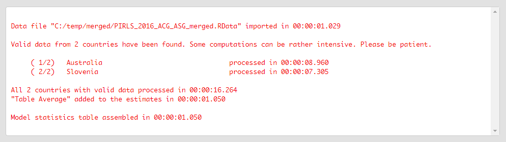
Executing the code from above will print the following output in the RStudio console:
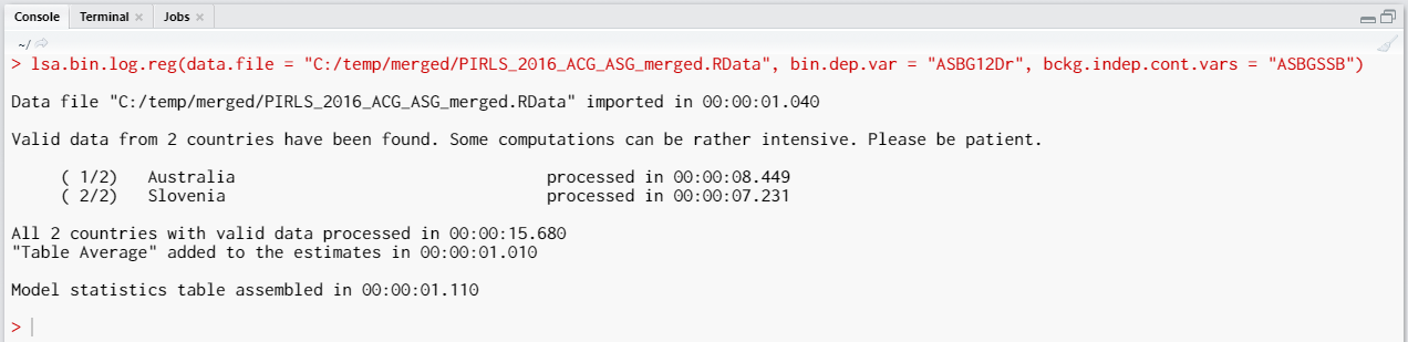
When all operations are finished the output will be written on the disk as MS Excel workbook. If open.output = TRUE (default), the file will be open in the default spreadsheet program (usually MS Excel). Refer to the explanations on the structure of the workbook, its sheets and the columns here.
Categorical variables can be added as contrast coded variables and the significance of the differences between the categories in the dependent variable can be tested. For now, the function can work with the following contrast schemes: dummy, deviation, and simple (see here for description). Let’s test the differences in log of the odds between female and male students when controlling for students’ sense of school belonging (ASBGSSB, check the PIRLS 2016 technical documentation on how this scale is constructed and its properties). This analysis extends the previous one, adding student gender (ASBG01) as categorical background variable to the bckg.indep.cat.vars argument of the function. The variable on student gender (ASBG01) has the two valid values:
- Girl
- Boy
We need to add ASBG01 as value of the bckg.indep.cat.vars argument of the lsa.bin.log.reg function. The function will automatically determine the valid values, but we need to specify the reference category as a values of the bckg.cat.contrasts (the type of contrast coding) and the bckg.ref.cat (the reference category). If we omit specifying a value for bckg.cat.contrasts (which we will), the function will automatically compute the regression coefficients with dummy coding (the intercept will be the log of the odds for the dependent variable for students falling into the category we have chosen as a reference, see further) and the regression coefficients for the rest of the categories (which is just one in this case because we have two genders) will be the differences in log of the odds for the students who fall into any other category, but the reference. If any other contrast scheme is needed, it has to be specified explicitly, using the bckg.cat.contrasts argument, see here. We will define the first category (“Girl”) as a reference. We will add students’ sense of school belonging (ASBGSSB, check the PIRLS 2016 technical documentation on how this scale is constructed and its properties) as a control variable as a value of bckg.indep.cont.vars. The calling syntax looks like this:
lsa.bin.log.reg(data.file = "C:/temp/merged/PIRLS_2016_ACG_ASG_merged.RData",
                bin.dep.var = "ASBG12Dr",
                bckg.indep.cont.vars = "ASBGSSB",
                bckg.indep.cat.vars = "ASBG01",
                bckg.ref.cats = 1)
Executing the syntax from above will overwrite the previous output because it has the same file name defined (a warning will be displayed in the console). The columns in the “Estimates” sheet will now be different. For the meaning of the column names, refer to the list here.
Computing binary logistic regression coefficients using the GUI
To start the RALSA user interface, execute the following command in RStudio:
ralsaGUI()
For the examples that follow, merge a new file with PIRLS 2016 data for Australia and Slovenia (Slovenia, not Slovakia) taking all student and school principal variables. See how to merge data files here. You can name the merged file PIRLS_2016_ACG_ASG_merged.RData.
As a start, let’s compute the binary logistic regression coefficients for a model to predict if students would agree or disagree that teachers treat them fair (variable ASBG12D) as a function of their own sense of school belonging (ASBGSSB, check the PIRLS 2016 technical documentation on how this scale is constructed and its properties) in Australia and Slovenia. Logistic regression accepts only binary (i.e. dichotomous) variables as dependent, while the responses on the question of how much students agree or disagree that teachers treat them fair (ASBG12D) are organized into four distinct categories:
- Agree a lot
- Agree a little
- Disagree a little
- Disagree a lot
Thus, the first thing we need to do is to recode ASBG12D collapsing the categories into two where the “Disagree a lot” and “Disagree a little” are recoded as the first category, and “Agree a lot” and “Agree a little” as the second category. To make the recodings, you need to recode the ASBG12D variable into a new one. Lets name it ASBG12Dr or under a name of your convenience. Navigate to Data preparation > Recode variables, load the merged file PIRLS_2016_ACG_ASG_merged.RData, and recode ASBG12D into ASBG12Dr, so that the “Disagree a lot” and “Disagree a little” are collapsed in one category (1 – “Disagree”) and “Agree a lot” and “Agree a little” in another category (2 – “Agree”). Do not forget to assign “Omitted or invalid” as a missing value. Check here to see how to recode variables in RALSA.
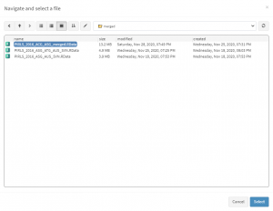
When done recoding the variable, select Analysis types > Binary logistic regression from the menu on the left. When navigated to the Binary logistic regression in the GUI, click on the Choose data file button. Navigate to the folder containing the merged PIRLS_2016_ACG_ASG_merged.RData file, select it and click the Select button.
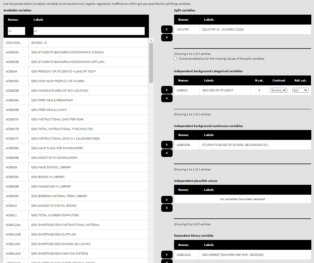
Once the file is loaded, you will see a panel on the left (available variables) and set of panels on the right where variables from the list of available ones can be added. Above the panels you will also see information about the loaded file.
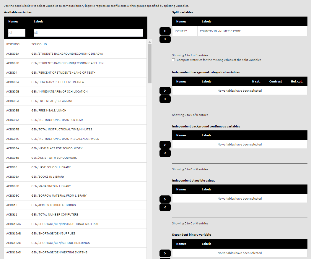
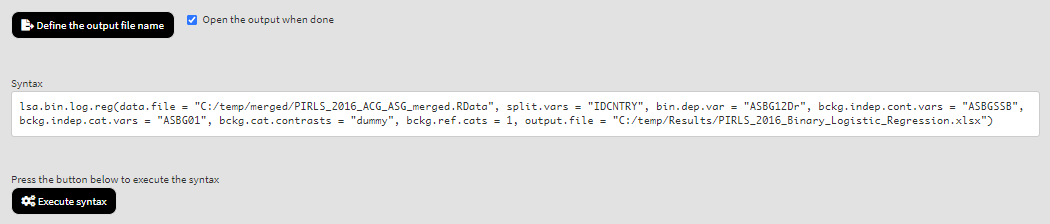
Use the mouse to select variables from the list of Available variables and the arrow buttons in the middle of the screen to add them to different fields (or remove them) to make the settings for the analysis. You can use the filter boxes on the top of the panels to find the needed variables quickly. Let’s compute the logistic regression coefficients using the new variable ad dependent and ASBGSSB as independent. Select the new recoded variable ASBG12Dr from the list of the Available variables and move it to the list of Dependent binary variable using the right arrow button. Select variable ASBGSSB in the list of Available variables and move it to the list of Independent background continuous variables using the right arrow button. This is all that needs to be done. Scroll down and click on the Define output file name. Navigate to the folder C:/temp/Results (or to the folder where you want to save the output) and define the output file name. After you do so, a checkbox will appear next to the Define the output file name. If ticked, the output will open after all computations are finished. Underneath you will see the Normalize the weights checkbox. If ticked, the weights will be normalized before used in the computations (see here for more details). You will also see the Standardized coefficients checkbox. If ticked, the variables will be standardized before the statistics is computed. See here for more details. Underneath the calling syntax will be displayed. Under all of these the Execute syntax button will be displayed. The final settings in the lower part of the screen should look like this:
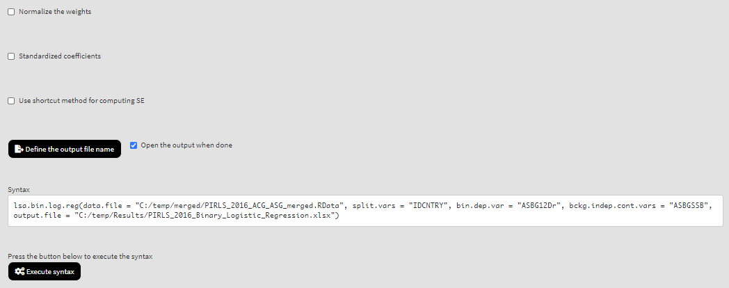
Click on the Execute syntax button. The GUI console will appear at the bottom and will log all completed operations:
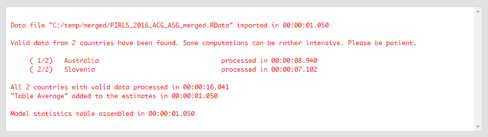
Few things to note:
- The function can take one binary variable as dependent. The independent variables can be multiple background/contextual variables and/or sets of PVs. If PVs are included as independent variables, each set of PVs will be represented by their root name. For example, the five PVs for the overall reading achievement are ASRREA01, ASRREA02, ASRREA03, ASRREA04, and ASRREA05. The root name of all PVs in a set will be shown in In the list of Available variables (or list of Independent plausible values, if selected there), in case of the overall reading achievement this will be ASRREA. The function will use this root/common name to select all five PVs and include them in the computations. For more details on the PV roots (also for the PV roots for studies other than TIMSS and PIRLS and their additions), the computational routines involving PVS, see here.
- In international large-scale assessments all analyses must be done separately by country. The country ID variable (IDCNTRY, or CNT in PISA) is always selected as the first splitting variable and cannot be removed from the Split variables panel.
- The default weight variable is selected and added automatically in the Weight variable panel. It can be changed with another weight variable available in the data set. If the default weight variable is selected, it will not be shown in the syntax window. If no weight variable is selected in the Weight variable panel, the default one will be used automatically.
- If the Standardized coefficients checkbox is ticked, the regression coefficients will be computed on standardized variables and beta coefficients will be included in the output.
- The Use shortcut method for computing SE checkbox is not ticked by default. This will make the function to compute the standard error using the “full” method for the sampling variance component. For more details see here and here.
If the Open the output when done checkbox is ticked, the output will open automatically in the default spreadsheet program (usually MS Excel) when all computations are completed. Refer to the explanations on the structure of the workbook, its sheets and the columns here.
Categorical variables can be added as contrast coded variables and the significance of the differences between the categories in the dependent variable can be tested. For now, the function can work with the following contrast schemes: dummy, deviation, and simple (see here for description). Let’s test the differences in log of the odds between female and male students when controlling for students’ sense of school belonging (ASBGSSB, check the PIRLS 2016 technical documentation on how this scale is constructed and its properties). This analysis extends the previous one, adding student gender (ASBG01) as categorical background variable to the list of Independent background categorical variables. The variable on student gender (ASBG01) has the two valid values:
- Girl
- Boy
Locate variable ASBG01 in the list of Available variables (you can use the filter box on the top), select it and add it to the list of Independent background categorical variables using the right arrow button. You will see that the list will automatically show the number of categories for the variable, a drop-down list with the different coding schemes (dummy, deviation and simple, see column N cat.), and the drop-down list with the variable’s categories to choose from:
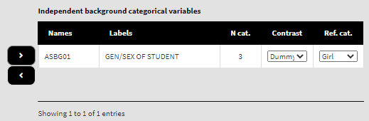
By default, dummy contrast coding scheme and the first available category as a reference are chosen. Let’s leave the defaults. The function will automatically compute the regression coefficients with dummy coding (the intercept will be the log of the odds for the dependent variable for students falling into the category we have chosen as a reference, see further) and the regression coefficients for the rest of the categories (which is just one in this case because we have two genders) will be the differences in log of the odds for the students who fall into any other category, but the reference. If any other contrast scheme is needed, it can be changed by clicking on the drop-down menu and selecting either deviation or simple (for description of the different contrast coding schemes see here). We will leave the first category (“Girl”) as a reference. We will leave the variable ASBGSSB as a control variable in the list of Independent background continuous variables:
Because we use the application with Binary logistic regression directly after performing the previous analysis, we still have the rest of the settings from the previous analysis done. There is no need to change any of the remaining settings, unless you want to. You could, though, change the output file name, otherwise it will be overwritten. Note that the displayed syntax will change, reflecting the inclusion of the ASBG01 as independent categorical variable:
Press the Execute syntax button. The GUI console will update, logging all completed operations:
If the Open the output when done checkbox is ticked, the output will open automatically in the default spreadsheet program (usually MS Excel) when all computations are completed. As with the previous analyses, refer to the explanations on the structure of the workbook, its sheets and the columns here.