
Table of contents
- Introduction
- The percentages and means function and its arguments
- Computing percentages and means using the command line
- Computing percentages and means using the GUI
Introduction
The lsa.pcts.means function computes percentages of respondents within groups of respondents defined by the categories of splitting variables and the means (arithmetic average, median or mode) of continuous variables within these groups. Both the splitting variables and the variables to compute the means are optional. If no splitting variables are provided, the results will be computed on country level only. If splitting variables are provided, the data within each country will be split into groups by all splitting variables and the percentages of respondents will be computed for the last splitting variable. If variables to compute means for are provided, their means within groups defined by all splitting variables will be computed. Note that the means can be computed for both background/contextual variables or sets of PVs, taking into account the complex sampling and assessment design of the study of interest. In the latter case, the means will be computed for each PV in a set, and then the estimates for all PVs in the set will be averaged and their standard error computed using complex formulas which will depend on the study of interest. Whatever the estimate is, the standard error will be computed taking into account the complex sampling and assessment designs of the studies. Refer here for a short overview on the complex sampling and assessment designs of large-scale assessments and surveys. If interested in more in-depth details on the complex sampling and assessment designs of a particular study and how estimates and their standard errors are computed, refer to its technical documentation and user guide.
Like any other function in the RALSA package, the lsa.pcts.means function can recognize the study data and apply the correct estimation techniques given the study sampling and assessment design implementation without extra care.
The percentages and means function and its arguments
The lsa.pcts.means function has the following arguments:
data.file– The file containinglsa.dataobject. Either this ordata.objectshall be specified, but not both.data.object– The object in the memory containinglsa.dataobject. Either this ordata.fileshall be specified, but not both.split.vars– Categorical variable(s) to split the results by. If no split variables are provided, the results will be for the overall countries’ populations. If one or more variables are provided, the results will be split by all but the last variable and the percentages of respondents will be computed by the unique values of the last splitting variable.bckg.avg.vars– Name(s) of continuous background or contextual variable(s) to compute the means for. The results will be computed by all groups specified by the splitting variables.PV.root.avg– The root name(s) for the set(s) of plausible values.central.tendency– Which measure of central tendency shall be computed –mean, (default)medianormode.weight.var– The name of the variable containing the weights. If no name of a weight variable is provide, the function will automatically select the default weight variable for the provided data, depending on the respondent type.include.missing– Logical, shall the missing values of the splitting variables be included as categories to split by and all statistics produced for them? The default (FALSE) takes all cases on the splitting variables without missing values before computing any statistics.shortcut– Logical, shall the “shortcut” method for IEA TIMSS, TIMSS Advanced, TIMSS Numeracy, eTIMSS, PIRLS, ePIRLS, PIRLS Literacy and RLII be applied? The default (FALSE) applies the “full” design when computing the variance components and the standard errors of the estimates.graphs– Logical, shall graphs be produced? Default isFALSE.perc.x.label– String, custom label for the horizontal axis in percentage graphs. Ignored ifgraphs = FALSE.perc.y.label– String, custom label for the vertical axis in percentage graphs. Ignored ifgraphs = FALSE.mean.x.labels– List of strings, custom labels for the horizontal axis in means’ graphs. Ignored ifgraphs = FALSE.mean.y.labels– List of strings, custom labels for the vertical axis in means’ graphs. Ignored ifgraphs = FALSE.save.output– Logical, shall the output be saved in MS Excel file (default) or not (printed to the console or assigned to an object).output.file– Full path to the output file including the file name. If omitted, a file with a default file name “Analysis.xlsx” will be written to the working directory (getwd()).open.output– Logical, shall the output be open after it has been written? The default (TRUE) opens the output in the default spreadsheet program installed on the computer.
Notes:
- Either
data.fileordata.objectshall be provided as source of data. If both of them are provided, the function will stop with an error message. The data must be of classlsa.data, these are converted from SPSS (or TXT in case of PISA prior to its 2015 cycle) using thelsa.convert.datafunction. - The function computes percentages of respondents specified by the categories of splitting variables. The percentages are computed within the groups specified by the last splitting variable. If a continuous variable(s) are provided (background or sets of plausible values), their means will be computed by groups defined by one or more splitting variables. If no splitting variables are added, the results will be computed only by country.
- Multiple continuous background variables can be provided to compute their means. Please note that in this case the results will slightly differ compared to using each of the same background continuous variables in separate analyses. This is because the cases with the missing values on
bckg.avg.varsare removed in advance and the more variables are provided tobckg.avg.vars, the more cases are likely to be removed. - Computation of means involving plausible values requires providing a root of the plausible values names in
PV.root.avg. All studies (except CivED, TEDS-M, SITES, TALIS and TALIS Starting Strong Survey) have a set of PVs per construct (e.g. in TIMSS five for overall mathematics, five for algebra, five for geometry, etc.). In some studies (say TIMSS and PIRLS) the names of the PVs in a set always start with character string and end with sequential number of the PV. For example, the names of the set of PVs for overall mathematics in TIMSS are BSMMAT01, BSMMAT02, BSMMAT03, BSMMAT04 and BSMMAT05. The root of the PVs for this set to be added toPV.root.avgwill be “BSMMAT”. The function will automatically find all the variables in this set of PVs and include them in the analysis. In other studies like OECD PISA and IEA ICCS and ICILS the sequential number of each PV is included in the middle of the name. For example, in ICCS the names of the set of PVs are PV1CIV, PV2CIV, PV3CIV, PV4CIV and PV5CIV. The root PV name has to be specified inPV.root.avgas “PV#CIV”. More than one set of PVs can be added. Note, however, that providing continuous variable(s) for thebckg.avg.varsargument and root PV for thePV.root.avgargument will affect the results for the PVs because the cases with missing onbckg.avg.varswill be removed and this will also affect the results from the PVs. On the other hand, using more than one set of PVs at the same time should not affect the results on any PV estimates because PVs shall not have any missing values. - If no variables are specified for
bckg.avg.vars, and no PV root names forPV.root.avg, the output will contain only percentages of cases in groups specified by the splitting variables, if any. - The default measure of central tendency is the arithmetic average (
mean). This can be changed tomedianormode. - If
include.missing = FALSE(default), all cases with missing values on the splitting variables will be removed and only cases with valid values will be retained in the statistics. Note that the data from the studies can be exported in two different ways: (1) setting all user-defined missing values to NA; and (2) importing all user-defined missing values as valid ones and adding their codes in an additional attribute to each variable. If theinclude.missingis set toFALSE(default) and the data used is exported using option (2), the output will remove all values from the variable matching the values in itsmissingsattribute. Otherwise, it will include them as valid values and compute statistics for them. - The
shortcutargument is valid only for TIMSS, TIMSS Advanced, TIMSS Numeracy, PIRLS, ePIRLS, PIRLS Literacy and RLII. Previously, in computing the standard errors, these studies were using 75 replicates because one of the schools in the 75 JK zones had its weights doubled and the other one has been taken out. Since TIMSS 2015 and PIRLS 2016 the studies use 150 replicates and in each JK zone once a school has its weights doubled and once taken out, i.e. the computations are done twice for each zone. For more details see the technical documentation and user guides for TIMSS 2015, and PIRLS 2016. If replication of the tables and figures is needed, the shortcut argument has to be changed toTRUE. - If graphs = TRUE, the function will produce graphs, bar plots for the percentages and error bars for the means per group defined by the
split.vars. All plots are produced per country. If nosplit.varsat the end there will be a percentages and error bar plots for all countries together. If needed, custom horizontal and vertical axis labels for the bar plots and error bar plots can be defined using theperc.x.label,perc.y.label,mean.x.labelsandmean.y.labelsarguments.
If save.output = FALSE, a list containing the estimates and analysis information. If graphs = TRUE, the plots will be added to the list of estimates.
If save.output = TRUE (default), an MS Excel (.xlsx) file (which can be opened in any spreadsheet program), as specified with the full path in the output.file. If the argument is missing, an Excel file with the generic file name “Analysis.xlsx” will be saved in the working directory (getwd()). The workbook contains three spreadsheets. The first one (“Estimates”) contains a table with the results by country and the final part of the table contains averaged results from all countries’ statistics. The following columns can be found in the table, depending on the specification of the analysis:
- <Country ID> – a column containing the names of the countries in the file for which statistics are computed. The exact column header will depend on the country identifier used in the particular study.
- <Split variable 1>, <Split variable 2>… – columns containing the categories by which the statistics were split by. The exact names will depend on the variables in
split.vars. - n_Cases – the number of cases in the sample used to compute the statistics.
- Sum_<Weight variable> – the estimated population number of elements per group after applying the weights. The actual name of the weight variable will depend on the weight variable used in the analysis.
- Sum_<Weight variable>_SE – the standard error of the the estimated population number of elements per group. The actual name of the weight variable will depend on the weight variable used in the analysis.
- Percentages_<Last split variable> – the percentages of respondents (population estimates) per groups defined by the splitting variables in
split.vars. The percentages will be for the last splitting variable which defines the final groups. - Percentages_<Last split variable>_SE – the standard errors of the percentages from above.
- Mean_<Background variable> – returned if
central.tendency = "mean", the average of the continuous <Background variable> specified inbckg.avg.vars. There will be one column with the average estimate for each variable specified inbckg.avg.vars. - Mean_<Background variable>_SE – returned if
central.tendency = "mean", the standard error of the average of the continuous <Background variable> specified inbckg.avg.vars. There will be one column with the SE of the average estimate for each variable specified inbckg.avg.vars. - Variance_<Background variable> – returned if
central.tendency = "mean", the variance for the continuous <Background variable> specified inbckg.avg.vars. There will be one column with the variance estimate for each variable specified inbckg.avg.vars. - Variance_<Background variable>_SE – returned if
central.tendency = "mean", the error of the variance for the continuous <Background variable> specified inbckg.avg.vars. There will be one column with the error of the variance estimate for each variable specified inbckg.avg.vars. - SD_<Background variable> – returned if
central.tendency = "mean", the standard deviation for the continuous <Background variable> specified inbckg.avg.vars. There will be one column with the standard deviation estimate for each variable specified inbckg.avg.vars. - SD_<Background variable>_SE – returned if
central.tendency = "mean", the error of the standard deviation for the continuous <Background variable> specified inbckg.avg.vars. There will be one column with the error of the standard deviation estimate for each variable specified inbckg.avg.vars. - Median_<Background variable> – returned if
central.tendency = "median", the median of the continuous <Background variable> specified inbckg.avg.vars. There will be one column with the median estimate for each variable specified inbckg.avg.vars. - Median_<Background variable>_SE – returned if
central.tendency = "median", the standard error of the median of the continuous <Background variable> specified inbckg.avg.vars. There will be one column with the SE of the median estimate for each variable specified inbckg.avg.vars. - MAD_<Background variable> – returned if
central.tendency = "median", the Median Absolute Deviation (MAD) for the continuous <Background variable> specified inbckg.avg.vars. There will be one column with the MAD estimate for each variable specified inbckg.avg.vars. - MAD_<Background variable>_SE – returned if
central.tendency = "median", the standard error of MAD for the continuous <Background variable> specified inbckg.avg.vars. There will be one column with the MAD SE estimate for each variable specified inbckg.avg.vars. - Mode_<Background variable> – returned if
central.tendency = "mode", the mode of the continuous <Background variable> specified inbckg.avg.vars. There will be one column with the mode estimate for each variable specified inbckg.avg.vars. - Mode_<Background variable>_SE – returned if
central.tendency = "mode", the standard error of the mode of the continuous <Background variable> specified inbckg.avg.vars. There will be one column with the SE of the mode estimate for each variable specified inbckg.avg.vars. - Percent_Missings_<Background variable> – the percentage of missing values for the <Background variable> specified in
bckg.avg.vars. There will be one column with the percentage of missing values for each variable specified inbckg.avg.vars. - Mean_<root PV> – returned if
central.tendency = "mean", the average of the PVs with the same <root PV> specified inPV.root.avg. There will be one column with the average estimate for each set of PVs specified inPV.root.avg. - Mean_<root PV>_SE – returned if
central.tendency = "mean", the standard error of the average of the PVs with the same <root PV> specified inPV.root.avg. There will be one column with the standard error of average estimate for each set of PVs specified inPV.root.avg. - Mean_<root PV>_SVR – returned if
central.tendency = "mean", the sampling variance component for the average of the PVs with the same <root PV> specified inPV.root.avg. There will be one column with the sampling variance component for the average estimate for each set of PVs specified inPV.root.avg. - Mean_<root PV>_MVR – returned if
central.tendency = "mean", the measurement variance component for the average of the PVs with the same <root PV> specified inPV.root.avg. There will be one column with the measurement variance component for the average estimate for each set of PVs specified inPV.root.avg. - Variance_<root PV> – returned if
central.tendency = "mean", the total variance of the PVs with the same <root PV> specified inPV.root.avg. There will be one column with the total variance of each set of PVs specified inPV.root.avg. - Variance_<root PV>_SE – returned if
central.tendency = "mean", the standard error of the total variance of the PVs with the same <root PV> specified inPV.root.avg. There will be one column with the standard error of the total variance of each set of PVs specified inPV.root.avg. - Variance_<root PV>_SVR – returned if
central.tendency = "mean", the sampling component of the variance of the PVs with the same <root PV> specified inPV.root.avg. There will be one column with the sampling component of the variance of each set of PVs specified inPV.root.avg. - Variance_<root PV>_MVR – returned if
central.tendency = "mean", the measurement component of the variance of the PVs with the same <root PV> specified inPV.root.avg. There will be one column with the measurement component of the variance of each set of PVs specified inPV.root.avg. - SD_<root PV> – returned if
central.tendency = "mean", the standard deviation of the PVs with the same <root PV> specified inPV.root.avg. There will be one column with the standard deviation of each set of PVs specified inPV.root.avg. - SD_<root PV>_SE – returned if
central.tendency = "mean", the standard error of the standard deviation of the PVs with the same <root PV> specified inPV.root.avg. There will be one column with the standard error of the standard deviation of each set of PVs specified inPV.root.avg. - SD_<root PV>_SVR – returned if
central.tendency = "mean", the sampling component of the standard deviation of the PVs with the same <root PV> specified inPV.root.avg. There will be one column with the sampling component of the standard deviation of each set of PVs specified inPV.root.avg. - SD_<root PV>_MVR – returned if
central.tendency = "mean", the measurement component of the standard deviation of the PVs with the same <root PV> specified inPV.root.avg. There will be one column with the measurement component of the standard deviation of each set of PVs specified inPV.root.avg. - Median_<root PV> – returned if
central.tendency = "median", the median of the PVs with the same <root PV> specified inPV.root.avg. There will be one column with the median estimate for each set of PVs specified inPV.root.avg. - Median_<root PV>_SE – returned if
central.tendency = "median", the standard error of the median of the PVs with the same <root PV> specified inPV.root.avg. There will be one column with the standard error of median estimate for each set of PVs specified inPV.root.avg. - MAD_<root PV> – returned if
central.tendency = "median", the Median Absolute Deviation (MAD) for a set of PVs specified inPV.root.avg. There will be one column with the MAD estimate for each set of PVs specified inPV.root.avg. - MAD_<root PV>_SE – returned if
central.tendency = "median", the standard error of MAD for a set of PVs specified inPV.root.avg. There will be one column with the SE estimate of the MAD for each set of PVs specified inPV.root.avg. - Mode_<root PV> – returned if
central.tendency = "mode", the mode of the PVs with the same <root PV> specified inPV.root.avg. There will be one column with the mode estimate for each set of PVs specified inPV.root.avg. - Mode_<root PV>_SE – returned if
central.tendency = "mode", the standard error of the mode of the PVs with the same <root PV> specified inPV.root.avg. There will be one column with the standard error of mode estimate for each set of PVs specified inPV.root.avg. - Percent_Missings_<root PV> – the percentage of missing values for the <root PV> specified in
PV.root.avg. There will be one column with the percentage of missing values for each set of PVs specified inPV.root.avg.
The second sheet (“Analysis information”) contains some additional information related to the analysis per country in the following columns:
- DATA – used
data.fileordata.object. - STUDY – which study the data comes from.
- CYCLE – which cycle of the study the data comes from.
- WEIGHT – which weight variable was used.
- DESIGN – which resampling technique was used (JRR or BRR).
- SHORTCUT – logical, whether the shortcut method was used.
- NREPS – how many replication weights were used.
- ANALYSIS_DATE – on which date the analysis was performed.
- START_TIME – at what time the analysis started.
- END_TIME – at what time the analysis finished.
- DURATION – how long the analysis took in hours, minutes, seconds and milliseconds.
The third sheet (“Calling syntax”) contains the call to the function with values for all parameters as it was executed. This is useful if the analysis needs to be replicated later.
If graphs = TRUE there will be an additional “Graphs” sheet containing all plots.
If any warnings resulting from the computations are issued, these will be included in an additional “Warnings” sheet in the workbook as well.
Computing percentages and means using the command line
In the examples that follow we will merge a new data file (see how to merge files here) with student and school principal data from PIRLS 2016 (Australia and Slovenia), taking all variables from both file types:
lsa.merge.data(inp.folder = "C:/temp",
               file.types = list(acg = NULL, asg = NULL),
               ISO = c("aus", "svn"),
               out.file = "C:/temp/merged/PIRLS_2016_ACG_ASG_merged.RData")
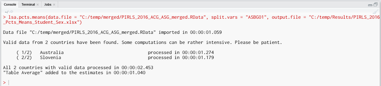
As a start, let’s compute the percentages of female and male students in Australia and Slovenia:
lsa.pcts.means(data.file = "C:/temp/merged/PIRLS_2016_ACG_ASG_merged.RData",
               split.vars = "ASBG01",
               output.file = "C:/temp/Results/PIRLS_2016_Pcts_Means_Student_Sex.xlsx")
Few things to note:
- There are two variables containing the information on student sex:
- ITSEX, a variable containing the student tracking information; and
- ASBG01 (used in this analysis), a variable containing the student sex as the students responded in the questionnaire.
- In international large-scale assessments all analyses must be done separately by country. There is no need, however, to add the country ID variable (IDCNTRY, or CNT in PISA) as a splitting variable. The function will identify it automatically and add it to the the vector of
split.vars. - The measure of central tendency was not explicitly specified. In this cese the arithmetic average (mean) was computed. To change the measure of central tendency, set the
central.tendencyargument tomedianormode. - There is no need to specify the weight variable explicitly. If no weight variable is specified explicitly, then the default weight (total student weight in this case) will be used for the data set depending on the merged respondents’ data, it is identified automatically. If you have a good reason to change the weight variable, you can do so by adding the
weight.var = "SENWGT", for example. - If no output file is specified, then the output will be saved with “Analysis.xlsx” file name under the working directory (can be obtained with
getwd()). - Unless explicitly adding
save.output = FALSE, the output will be written to MS Excel on the disk. Otherwise, the output will be printed to the console. - Unless explicitly adding
open.output = FALSE, to the calling syntax, the output file will be opened after all computations are finished. This is useful when multiple calling syntaxes for different analyses are executed and no immediate inspection of the output is needed.
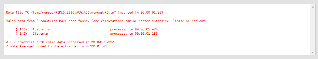
Executing the code from above will print the following output in the RStudio console:
When all operations are finished the output will be written on the disk as MS Excel workbook. If open.output = TRUE (default), the file will be open in the default spreadsheet program (usually MS Excel). Refer to the explanations on the structure of the workbook, its sheets and the columns here.
Let’s compute the averages of a variable for girls and boys. We will use the complex scale on how much students like reading (ASBGSLR, check the PIRLS 2016 technical documentation on how this scale is constructed and its properties):
lsa.pcts.means(data.file = "C:/temp/merged/PIRLS_2016_ACG_ASG_merged.RData",
               split.vars = "ASBG01",
               bckg.avg.vars = "ASBGSLR",
               output.file = "C:/temp/Results/PIRLS_2016_Pcts_Means_Student_Sex.xlsx")
The calling syntax from above adds the bckg.avg.vars and its value, the variable name ASBGSLR. The output has similar structure to the previous one, except that this time the columns pertinent to the mean for the scale are added.
The function can also compute the mean for a set (or sets) of plausible values. The calling syntax below computes the average overall reading achievement for boys and girls:
lsa.pcts.means(data.file = "C:/temp/merged/PIRLS_2016_ACG_ASG_merged.RData",
               split.vars = "ASBG01", PV.root.avg = "ASRREA",
               output.file = "C:/temp/Results/PIRLS_2016_Pcts_Means_Student_Sex.xlsx")
Note how the PVs are specified. The five PVs for the overall reading achievement are ASRREA01, ASRREA02, ASRREA03, ASRREA04, and ASRREA05. In the PV.root.avg argument we need to specify only the root of the PVs, “ASRREA”. The function will use this root/common name to select all five PVs and include them in the computations. For more details on the PV roots (also for the PV roots for studies other than TIMSS and PIRLS and their additions), the computational routines involving PVS, see here.
Executing the syntax from above will overwrite the previous output because it has the same file name defined (a warning will be displayed in the console). The columns in the “Estimates” sheet will now be different. For the meaning of the column names, refer to the list here.
Computing percentages and means using the GUI
To start the RALSA user interface, execute the following command in RStudio:
ralsaGUI()
For the examples that follow, merge a new file with PIRLS 2016 data for Australia and Slovenia (Slovenia, not Slovakia) taking all student and school principal variables. See how to merge data files here. You can name the merged file PIRLS_2016_ACG_ASG_merged.RData.
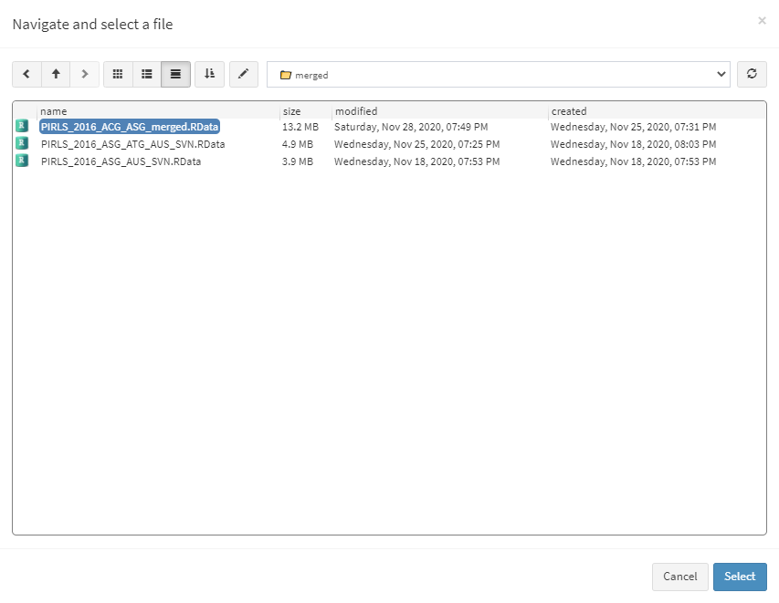
When done merging the data, select Analysis types > Percentages and means from the menu on the left. When navigated to the Percentages and means in the GUI, click on the Choose data file button. Navigate to the folder containing the merged PIRLS_2016_ACG_ASG_merged.RData file, select it and click the Select button.
Once the file is loaded, you will see a panel on the left (available variables) and set of panels on the right where variables from the list of available ones can be added.
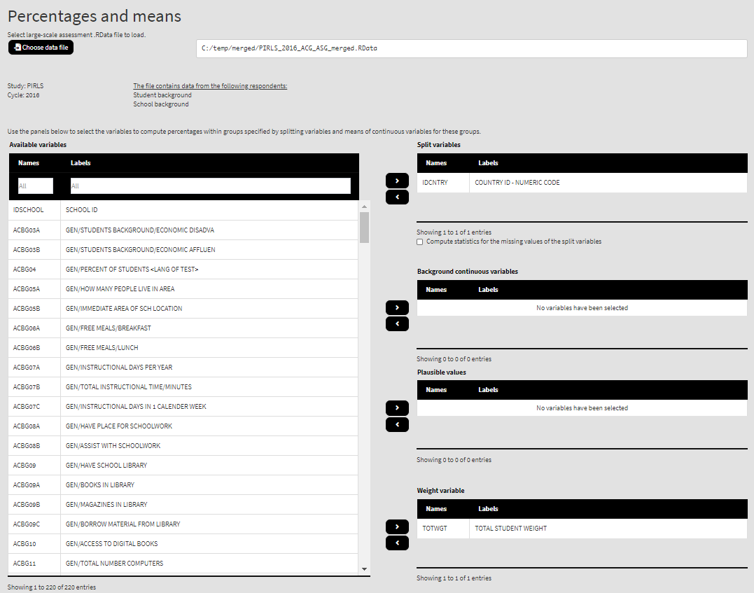
Use the mouse to select variables from the list of Available variables and the arrow buttons in the middle of the screen to add them to different fields (or remove them) to make the settings for the analysis. You can use the filter boxes on the top of the panels to find the needed variables quickly.
As a start, let’s compute the percentages of female and male students in Australia and Slovenia. Select the variable ASBG01 from the list of Available variables and add them to the list of Split variables using the right arrow button. This is all that needs to be done. Scroll down and click on the Define output file name. Navigate to the folder C:/temp/Results (or to the folder where you want to save the output) and define the output file name. After you do so, a checkbox will appear next to the Define the output file name. If ticked, the output will open after all computations are finished. Underneath the calling syntax will be displayed. Under all of these the Execute syntax button will be displayed. The final settings in the lower part of the screen should look like this:

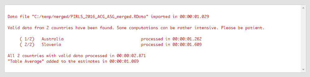
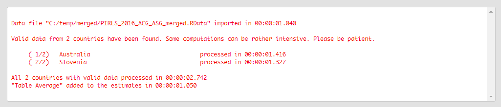
Click on the Execute syntax button. The GUI console will appear at the bottom and will log all completed operations:
Few things to note:
- There are two variables containing the information on student sex:
- ITSEX, a variable containing the student tracking information; and
- ASBG01 (used in this analysis), a variable containing the student sex as the students responded in the questionnaire.
- In international large-scale assessments all analyses must be done separately by country. The country ID variable (IDCNTRY, or CNT in PISA) is always selected as the first splitting variable and cannot be removed from the Split variables panel.
- The default weight variable is selected and added automatically in the Weight variable panel. It can be changed with another weight variable available in the data set. If the default weight variable is selected, it will not be shown in the syntax window. If no weight variable is selected in the Weight variable panel, the default one will be used automatically.
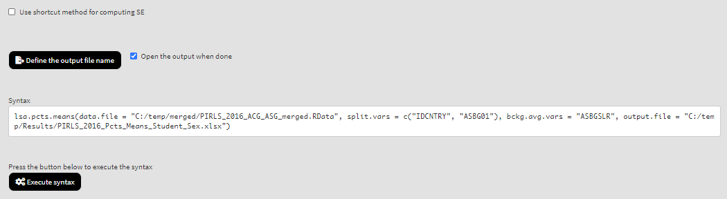
- The Use shortcut method for computing SE checkbox is not ticked by default. This will make the function to compute the standard error using the “full” method for the sampling variance component. For more details see here and here.
If the Open the output when done checkbox is ticked, the output will open automatically in the default spreadsheet program (usually MS Excel) when all computations are completed. Refer to the explanations on the structure of the workbook, its sheets and the columns here.
Let’s compute the averages for a variable for both girls and boys. We will use the complex scale on how much students like reading (ASBGSLR, check the PIRLS 2016 technical documentation on how this scale is constructed and its properties). Having made the settings for the previous analysis, select the variable ASBGSLR from the list of Available variables and use the arrow buttons to add it in the panel of Background continuous variables. Now the settings shall involve IDCNTRY and ASBG01 as Split variables and ASBGSLR as Background continuous variables:

Because we use the application with Percentages and means directly after performing the previous analysis, we still have the rest of the settings from the previous analysis done. There is no need to change any of the remaining settings, unless you want to. You could, though, change the output file name, otherwise it will be overwritten. Note that the displayed syntax will change, reflecting the inclusion of the ASBGSLR as a background continuous variable to compute the mean for:
Press the Execute syntax button. The GUI console will update, logging all completed operations:
After all computations are completed, the output will open automatically.
The function can also compute the mean for a set (or sets) of plausible values. To continue, select the ASBGSLR variable from the Background continuous variables panel and return it to the list of Available variables by clicking on the left arrow button. From the list of Available variables locate the root of the overall reading plausible values (ASRREA). You can use the filter boxes at the top of the panel to search for it, either by name or label. Select the root and add it to the Plausible values panel using the arrow buttons. This section of the interface should look like this:
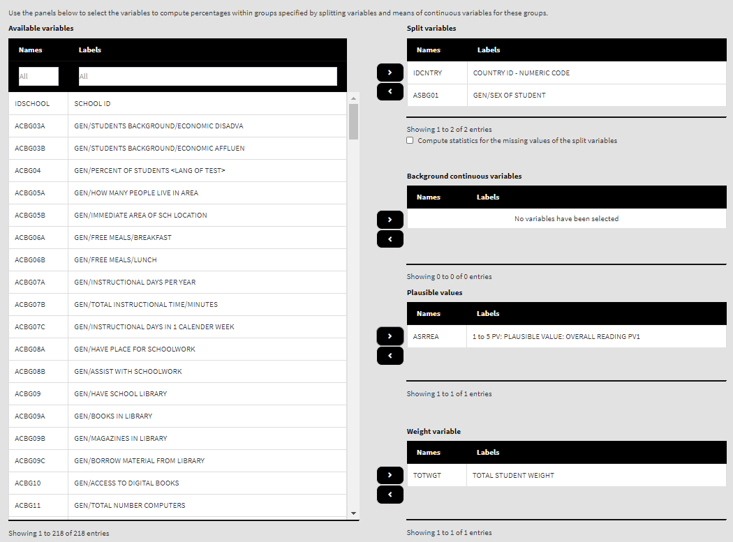
Note how the PVs are specified. The five PVs for the overall reading achievement are ASRREA01, ASRREA02, ASRREA03, ASRREA04, and ASRREA05. The lists of Available variables and Plausible values will not show the five separate PVs, but just their root/common name – ASRREA, without the numbers at the end. In the background, the function will take all the five PVs and include them in the computations. For more details on the PV roots (also for the PV roots for studies other than TIMSS and PIRLS and their additions), the computational routines involving PVS, see here.
Also, note that the measure of central tendency is arithmetic average (mean). It could be changed to median or mode using the radiobuttons directly underneath the panels for selecting variables:

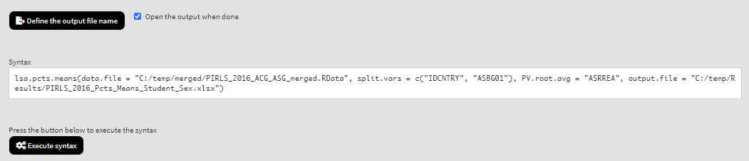
Because we use the application with Percentages and means directly after performing the previous analysis, we still have the rest of the settings from the previous analysis done. There is no need to change any of the remaining settings, unless you want to. You could, though, change the output file name, otherwise it will be overwritten. Note that the displayed syntax will change, reflecting the inclusion of the root of the five PVs, ASRREA, for the overall reading achievement to compute the mean for:
Press the Execute syntax button. The GUI console will update, logging all completed operations:
If the Open the output when done checkbox is ticked, the output will open automatically in the default spreadsheet program (usually MS Excel) when all computations are completed. As with the previous analyses, refer to the explanations on the structure of the workbook, its sheets and the columns here.